172 Computational Modelling in Hydraulic and Coastal Engineering
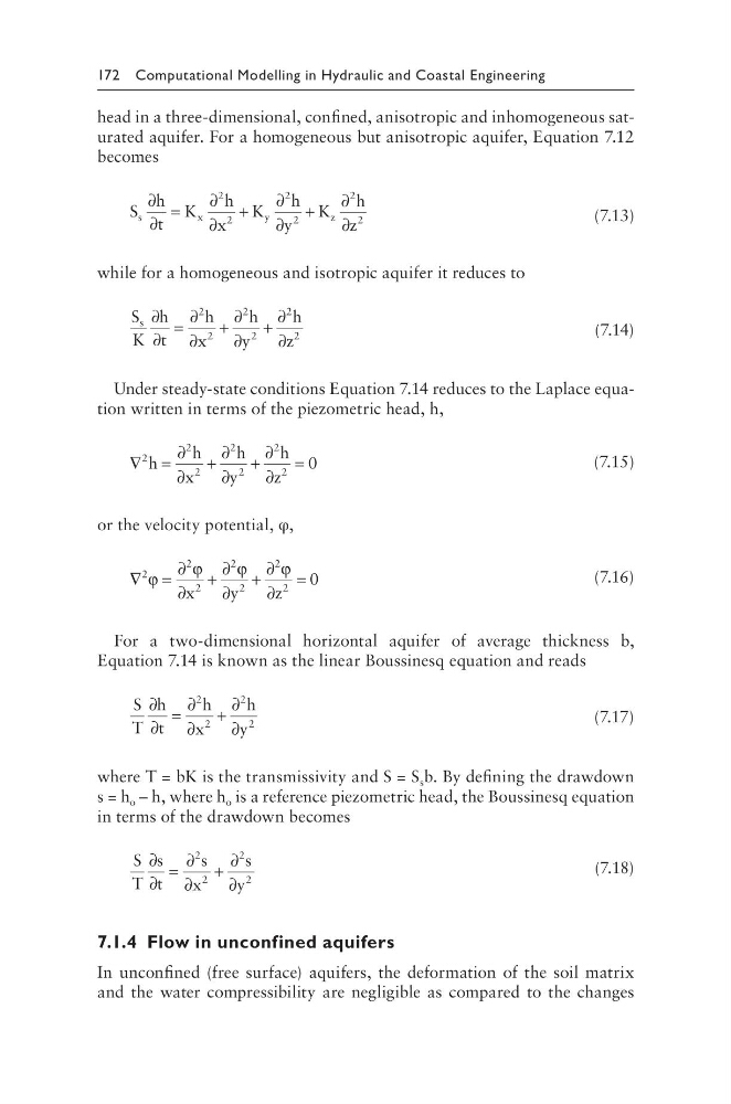
head in a three-dimensional, confined, anisotropic and inhomogeneous saturated aquifer. For a homogeneous but anisotropic aquifer, Equation 7.12
becomes
S
h
t
K
h
x
K
h
y
K
h
z
s
x
y
z
∂
∂
=
∂
∂
+
∂
∂
+
∂
∂
2
2
2
2
2
2
(7.13)
while for a homogeneous and isotropic aquifer it reduces to
S
K
h
t
h
x
h
y
h
z
s ∂
∂
=
∂
∂
+
∂
∂
+
∂
∂
2
2
2
2
2
2
(7.14)
Under steady-state conditions Equation 7.14 reduces to the Laplace equation written in terms of the piezometric head, h,
∇ =
∂
∂
+
∂
∂
+
∂
∂
=
2
2
2
2
2
2
2
0
h
h
x
h
y
h
z
(7.15)
or the velocity potential, φ,
∇ =
∂
∂
+
∂
∂
+
∂
∂
=
2
2
2
2
2
2
2
0
ϕ
ϕ
ϕ
ϕ
x
y
z
(7.16)
For a two-dimensional horizontal aquifer of average thickness b,
Equation 7.14 is known as the linear Boussinesq equation and reads
S
T
h
t
h
x
h
y
∂
∂
=
∂
∂
+
∂
∂
2
2
2
2
(7.17)
where T = bK is the transmissivity and S = S s b. By defining the drawdown
s = h o – h, where h o is a reference piezometric head, the Boussinesq equation
in terms of the drawdown becomes
S
T
s
t
s
x
s
y
∂
∂
=
∂
∂
+
∂
∂
2
2
2
2
(7.18)
7.1.4 Flow in unconfined aquifers
In unconfined (free surface) aquifers, the deformation of the soil matrix
and the water compressibility are negligible as compared to the changes