

Flow in porous media 175
7.2 NUMERICAL SOLUTIONS OF GROUNDWATER
FLOW APPLICATIONS
7.2.1 Steady-state vertical two- dimensional
groundwater flows
In the case of vertical two-dimensional steady-state flow, the governing
equation is the Laplace equation. By using a four-point finite differences
scheme, the discretized equation in terms of the velocity potential is similar
to that of Equation 3.16 (see Chapter 3):
ϕ
ϕ
ϕ
ϕ
ϕ
i j
i j
i j
i j
i j
,
,
,
,
,
(
)
=
+
+
+
+
−
+
−
1
4
1
1
1
1
(7.27)
Equation 7.27 can be solved very efficiently by using an iterative ‘relaxation’ procedure such as the Gauss-Seidel method. For confined flows, the
boundary conditions are fixed and predetermined. For unconfined flows,
the geometry of the water table has to be determined using the free surface
boundary condition. The discretization of the free surface boundary can
be accomplished by means of an explicit forward finite differences scheme,
according to the notations shown in Figure 7.2, as
h
h
t
K
n
h
h
s
n
i j
n
i j
n
e
i s
n
i j
n
e
i s
n
i
,
,
,
,
,
,
+
−
= −
−
= −
−
1
1
∆
∆
ϕ
ϕ j j
n
s
∆
(7.28)
where n is the time iteration number.
Therefore, for unconfined aquifers the solution involves an elliptic equation for the interior domain (Equation 7.27) and a hyperbolic equation for
the free surface (Equation 7.28). On the lateral solid boundaries, either the
D
ˆ
n
Impervious
boundary
(HAGI)
z 2
z
z 1
z o
y t
y 2
y 1
y o
C
Seepage surface (EF)
Free surface (phreatic) (BE)
G
F
E
B
A
Reference datum
I
H
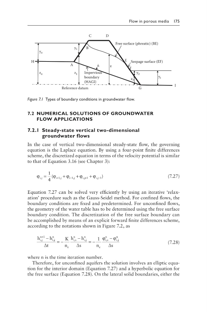
Figure 7.1 Types of boundary conditions in groundwater flow.
7.2 NUMERICAL SOLUTIONS OF GROUNDWATER
FLOW APPLICATIONS
7.2.1 Steady-state vertical two- dimensional
groundwater flows
In the case of vertical two-dimensional steady-state flow, the governing
equation is the Laplace equation. By using a four-point finite differences
scheme, the discretized equation in terms of the velocity potential is similar
to that of Equation 3.16 (see Chapter 3):
ϕ
ϕ
ϕ
ϕ
ϕ
i j
i j
i j
i j
i j
,
,
,
,
,
(
)
=
+
+
+
+
−
+
−
1
4
1
1
1
1
(7.27)
Equation 7.27 can be solved very efficiently by using an iterative ‘relaxation’ procedure such as the Gauss-Seidel method. For confined flows, the
boundary conditions are fixed and predetermined. For unconfined flows,
the geometry of the water table has to be determined using the free surface
boundary condition. The discretization of the free surface boundary can
be accomplished by means of an explicit forward finite differences scheme,
according to the notations shown in Figure 7.2, as
h
h
t
K
n
h
h
s
n
i j
n
i j
n
e
i s
n
i j
n
e
i s
n
i
,
,
,
,
,
,
+
−
= −
−
= −
−
1
1
∆
∆
ϕ
ϕ j j
n
s
∆
(7.28)
where n is the time iteration number.
Therefore, for unconfined aquifers the solution involves an elliptic equation for the interior domain (Equation 7.27) and a hyperbolic equation for
the free surface (Equation 7.28). On the lateral solid boundaries, either the
D
ˆ
n
Impervious
boundary
(HAGI)
z 2
z
z 1
z o
y t
y 2
y 1
y o
C
Seepage surface (EF)
Free surface (phreatic) (BE)
G
F
E
B
A
Reference datum
I
H
Figure 7.1 Types of boundary conditions in groundwater flow.