

140 Computational Modelling in Hydraulic and Coastal Engineering
λ is a dimensional coefficient (s –1 ). Furthermore, the energy dissipation in
the breaker zone due to turbulence can be modelled by introducing a term
in the right-hand side of Equation 6.17 in the form of N t x
b
∂
∂
∂
∂
2
2
ζ . The
magnitude of the coefficient N b is in the order of
1
2
h gh and its physical
significance is analogous to the horizontal eddy viscosity coefficient.
6.2.2 Discretization of the wave equation
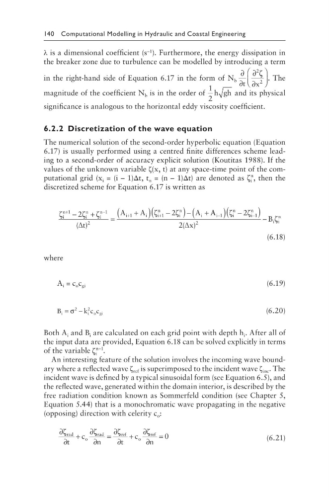
The numerical solution of the second-order hyperbolic equation (Equation
6.17) is usually performed using a centred finite differences scheme leading to a second-order of accuracy explicit solution (Koutitas 1988). If the
values of the unknown variable ζ(x, t) at any space-time point of the computational grid (x i = (i – 1)Δt, t n = (n – 1)Δt) are denoted as ζ i
n
, then the
discretized scheme for Equation 6.17 is written as
ζ
ζ ζ
ζ
ζ
i
n
i
n
i
n
i
i
i
n
i
n
i
t
A
A
A
+
−
+
+
−
+
=
+
(
) −
(
)− +
1
1
2
1
1
2
2
( )
∆
A A
x
B
i
i
n
i
n
i i
n
−
−
(
) −
(
) −
1
1
2
2
2
ζ
ζ
ζ
( )
∆
(6.18)
where
A i = c o c gi
(6.19)
B
kc c
i
io gi
=
−
σ
2
2
(6.20)
Both A i and B i are calculated on each grid point with depth h i . After all of
the input data are provided, Equation 6.18 can be solved explicitly in terms
of the variable ζ i
n+1
.
An interesting feature of the solution involves the incoming wave boundary where a reflected wave ζ ref is superimposed to the incident wave ζ inc . The
incident wave is defined by a typical sinusoidal form (see Equation 6.5), and
the reflected wave, generated within the domain interior, is described by the
free radiation condition known as Sommerfeld condition (see Chapter 5,
Equation 5.44) that is a monochromatic wave propagating in the negative
(opposing) direction with celerity c o :
∂
∂
+
∂
∂
=
∂
∂
+
∂
∂
=
ζ
ζ
ζ
ζ
rad
o
rad
r ef
o
ref
t
c
n
t
c
n
0
(6.21)
λ is a dimensional coefficient (s –1 ). Furthermore, the energy dissipation in
the breaker zone due to turbulence can be modelled by introducing a term
in the right-hand side of Equation 6.17 in the form of N t x
b
∂
∂
∂
∂
2
2
ζ . The
magnitude of the coefficient N b is in the order of
1
2
h gh and its physical
significance is analogous to the horizontal eddy viscosity coefficient.
6.2.2 Discretization of the wave equation
The numerical solution of the second-order hyperbolic equation (Equation
6.17) is usually performed using a centred finite differences scheme leading to a second-order of accuracy explicit solution (Koutitas 1988). If the
values of the unknown variable ζ(x, t) at any space-time point of the computational grid (x i = (i – 1)Δt, t n = (n – 1)Δt) are denoted as ζ i
n
, then the
discretized scheme for Equation 6.17 is written as
ζ
ζ ζ
ζ
ζ
i
n
i
n
i
n
i
i
i
n
i
n
i
t
A
A
A
+
−
+
+
−
+
=
+
(
) −
(
)− +
1
1
2
1
1
2
2
( )
∆
A A
x
B
i
i
n
i
n
i i
n
−
−
(
) −
(
) −
1
1
2
2
2
ζ
ζ
ζ
( )
∆
(6.18)
where
A i = c o c gi
(6.19)
B
kc c
i
io gi
=
−
σ
2
2
(6.20)
Both A i and B i are calculated on each grid point with depth h i . After all of
the input data are provided, Equation 6.18 can be solved explicitly in terms
of the variable ζ i
n+1
.
An interesting feature of the solution involves the incoming wave boundary where a reflected wave ζ ref is superimposed to the incident wave ζ inc . The
incident wave is defined by a typical sinusoidal form (see Equation 6.5), and
the reflected wave, generated within the domain interior, is described by the
free radiation condition known as Sommerfeld condition (see Chapter 5,
Equation 5.44) that is a monochromatic wave propagating in the negative
(opposing) direction with celerity c o :
∂
∂
+
∂
∂
=
∂
∂
+
∂
∂
=
ζ
ζ
ζ
ζ
rad
o
rad
r ef
o
ref
t
c
n
t
c
n
0
(6.21)