

Surface gravity water waves 139
6.2.1 Linearization of the governing equations
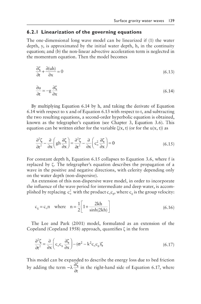
The one-dimensional long wave model can be linearized if (1) the water
depth, y, is approximated by the initial water depth, h, in the continuity
equation; and (b) the non-linear advective acceleration term is neglected in
the momentum equation. Then the model becomes
∂
∂
+
∂
∂
=
ζ
t
uh
x
( ) 0
(6.13)
∂
∂
= −
∂
∂
u
t
g x
ζ
(6.14)
By multiplying Equation 6.14 by h, and taking the derivate of Equation
6.14 with respect to x and of Equation 6.13 with respect to t, and subtracting
the two resulting equations, a second-order hyperbolic equation is obtained,
known as the telegrapher’s equation (see Chapter 3, Equation 3.6). This
equation can be written either for the variable ζ(x, t) (or for the u(x, t)) as
∂
∂
−
∂
∂
∂
∂
=
∂
∂
−
∂
∂
∂
∂
=
2
2
2
2
2
ζ
ζ
ζ
ζ
t
x
gh x
t
x
c x
o
0 0
(6.15)
For constant depth h, Equation 6.15 collapses to Equation 3.6, where f is
replaced by ζ. The telegrapher’s equation describes the propagation of a
wave in the positive and negative directions, with celerity depending only
on the water depth (non-dispersive).
An extension of this non-dispersive wave model, in order to incorporate
the influence of the wave period for intermediate and deep water, is accomplished by replacing c o
2
with the product c o c g , where c g is the group velocity:
c c n where n
kh
kh
g
o
=
=
+
1
2
1
2
2
sinh(
)
(6.16)
The Lee and Park (2001) model, formulated as an extension of the
Copeland (Copeland 1958) approach, quantifies ζ in the form
∂
∂
=
∂
∂
∂
∂
−
−
2
2
2
2
ζ
ζ
σ
ζ
t
x
c c x
k c c
o g
o g
(
)
(6.17)
This model can be expanded to describe the energy loss due to bed friction
by adding the term −
∂
∂
λ
ζ
t
in the right-hand side of Equation 6.17, where
6.2.1 Linearization of the governing equations
The one-dimensional long wave model can be linearized if (1) the water
depth, y, is approximated by the initial water depth, h, in the continuity
equation; and (b) the non-linear advective acceleration term is neglected in
the momentum equation. Then the model becomes
∂
∂
+
∂
∂
=
ζ
t
uh
x
( ) 0
(6.13)
∂
∂
= −
∂
∂
u
t
g x
ζ
(6.14)
By multiplying Equation 6.14 by h, and taking the derivate of Equation
6.14 with respect to x and of Equation 6.13 with respect to t, and subtracting
the two resulting equations, a second-order hyperbolic equation is obtained,
known as the telegrapher’s equation (see Chapter 3, Equation 3.6). This
equation can be written either for the variable ζ(x, t) (or for the u(x, t)) as
∂
∂
−
∂
∂
∂
∂
=
∂
∂
−
∂
∂
∂
∂
=
2
2
2
2
2
ζ
ζ
ζ
ζ
t
x
gh x
t
x
c x
o
0 0
(6.15)
For constant depth h, Equation 6.15 collapses to Equation 3.6, where f is
replaced by ζ. The telegrapher’s equation describes the propagation of a
wave in the positive and negative directions, with celerity depending only
on the water depth (non-dispersive).
An extension of this non-dispersive wave model, in order to incorporate
the influence of the wave period for intermediate and deep water, is accomplished by replacing c o
2
with the product c o c g , where c g is the group velocity:
c c n where n
kh
kh
g
o
=
=
+
1
2
1
2
2
sinh(
)
(6.16)
The Lee and Park (2001) model, formulated as an extension of the
Copeland (Copeland 1958) approach, quantifies ζ in the form
∂
∂
=
∂
∂
∂
∂
−
−
2
2
2
2
ζ
ζ
σ
ζ
t
x
c c x
k c c
o g
o g
(
)
(6.17)
This model can be expanded to describe the energy loss due to bed friction
by adding the term −
∂
∂
λ
ζ
t
in the right-hand side of Equation 6.17, where