

Free surface flows 119
The simulation period was sufficient for the establishment of
steady-state conditions. As can be seen from the time evolution of the
total kinetic energy graph (Figure 5.17), steady-state conditions were
reached after about 11,520 time steps (4 days).
The effects of the continuously blowing northwestern wind result
into the creation of two distinct large-scale clockwise vortices generating a northbound current drift along the west coast and a southbound
drift along the east coast of the gulf (Figure 5.18).
The three-dimensional nature of the flow in such sea basins is sometimes important, and particularly in the case of wind-generated currents. In order to avoid the application of 3-D models, one can adopt
a functional form of the velocity variation along the depth (a typical
velocity profile) and deduce the local velocities U(x,y,z,t), V(x,y,z,t)
from their depth mean values u(x,y,t), v(x,y,t), the water depth h(x,y)
and the wind friction τ sx , τ sy (functions of w x , w y ). If a parabolic velocity distribution is assumed, then the following relations can be applied
for the velocity U (Koutitas and Gousidou-Koutita 1986):
U = α 1 z 2 + α 2 z + α 3 where −h ≤ z ≤ 0
(5.59)
where the coefficients α 1 , α 2 and α 3 are defined as
α
τ
ρε
1
2
3
4
3
2
=
−
h
u
h
sx
h
(5.60)
0
–50
–100
–150
30
20
10
0 0
5
10
15
20
25
0
–10
–20
–30
–40
–50
–60
–70
–80
–90
–100
–110
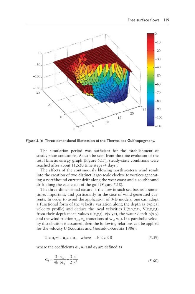
Figure 5.16 Three-dimensional illustration of the Thermaikos Gulf topography.
The simulation period was sufficient for the establishment of
steady-state conditions. As can be seen from the time evolution of the
total kinetic energy graph (Figure 5.17), steady-state conditions were
reached after about 11,520 time steps (4 days).
The effects of the continuously blowing northwestern wind result
into the creation of two distinct large-scale clockwise vortices generating a northbound current drift along the west coast and a southbound
drift along the east coast of the gulf (Figure 5.18).
The three-dimensional nature of the flow in such sea basins is sometimes important, and particularly in the case of wind-generated currents. In order to avoid the application of 3-D models, one can adopt
a functional form of the velocity variation along the depth (a typical
velocity profile) and deduce the local velocities U(x,y,z,t), V(x,y,z,t)
from their depth mean values u(x,y,t), v(x,y,t), the water depth h(x,y)
and the wind friction τ sx , τ sy (functions of w x , w y ). If a parabolic velocity distribution is assumed, then the following relations can be applied
for the velocity U (Koutitas and Gousidou-Koutita 1986):
U = α 1 z 2 + α 2 z + α 3 where −h ≤ z ≤ 0
(5.59)
where the coefficients α 1 , α 2 and α 3 are defined as
α
τ
ρε
1
2
3
4
3
2
=
−
h
u
h
sx
h
(5.60)
0
–50
–100
–150
30
20
10
0 0
5
10
15
20
25
0
–10
–20
–30
–40
–50
–60
–70
–80
–90
–100
–110
Figure 5.16 Three-dimensional illustration of the Thermaikos Gulf topography.