

120 Computational Modelling in Hydraulic and Coastal Engineering
α
τ
ρε
2 =
sx
h
(5.61)
α
ε
τ
ρ
3
4
3
2
=
+
h
u
h
sx
(5.62)
Similarly the equations for V are
V = β 1 z 2 + β 2 z + β 3 where −h ≤ z ≤ 0
(5.63)
β
τ
ρε
1
2
3
4
3
2
=
−
h
v
h
sy
h
(5.64)
β
τ
ρε
2 =
sy
h
(5.65)
β
ε
τ
ρ
3
4
3
2
=
+
h
v
h
sy
(5.66)
0.7
0.6
0.5
0.4
0.3
0.2
0.1
0 0
0.5
1
1.5
2
2.5
Number of time steps
× 10 4
Total kinetic energy (u 2
+v 2
on all grid points)
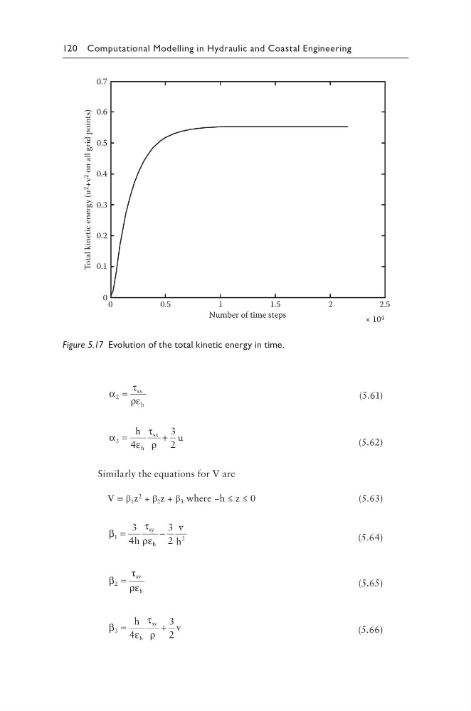
Figure 5.17 Evolution of the total kinetic energy in time.
α
τ
ρε
2 =
sx
h
(5.61)
α
ε
τ
ρ
3
4
3
2
=
+
h
u
h
sx
(5.62)
Similarly the equations for V are
V = β 1 z 2 + β 2 z + β 3 where −h ≤ z ≤ 0
(5.63)
β
τ
ρε
1
2
3
4
3
2
=
−
h
v
h
sy
h
(5.64)
β
τ
ρε
2 =
sy
h
(5.65)
β
ε
τ
ρ
3
4
3
2
=
+
h
v
h
sy
(5.66)
0.7
0.6
0.5
0.4
0.3
0.2
0.1
0 0
0.5
1
1.5
2
2.5
Number of time steps
× 10 4
Total kinetic energy (u 2
+v 2
on all grid points)
Figure 5.17 Evolution of the total kinetic energy in time.