

260
CONTINUOUS SYSTEMS
buoy involved. A way to calculate û> for a moored barge is discussed in Section
10.4. Neglect ail damping and ail transverse loading except at x = £ The model
for transverse cable motion is assumed as équation (10.13), for which a steady
State solution is chosen in the same form as for the end excitation imposed at
x = t, or
v(x, t) = X cos coi
(10.52)
where X = X(x). Combine équation (10.52) with (10.13) from which
X" + 72X = 0
(10.53)
o
m o
’’’ = PÔW
The general solution to équation (10.53) is given by
X — £>i sin yx + £>2 cos 72:
(10.54)
(10.55)
Applying the fixed boundary condition of équation (10.50) to (10.52), then
X(0) = 0. This same condition applied to équation (10.55) gives
= 0.
Combining équation (10.52) with (10.55), and that resuit with the other end
condition, équation (10.51) leads to
— Di sin 7^ cos wt = «o coswt
(10.56a)
Dr =
(10.56b)
sin 7e
From équation (10.54) and the expression for the natural frequencies un given
by équation (10.22), it follows that
7« =
= ntr(10.57)
y/Po/m
u>„
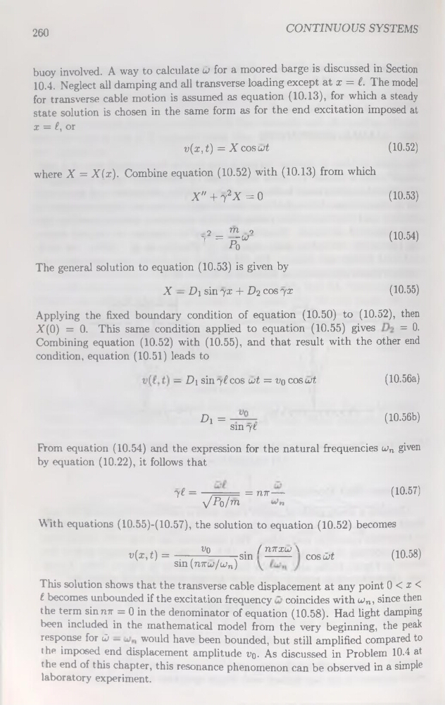
With équations (10.55)-(10.57), the solution to équation (10.52) becomes
v(x,t) = ■. , V° .—7 sin
sin (n7rw/con)
( mïxuj \
COSÛli
(10.58)
This solution shows that the transverse cable displacement at any point 0 < x <
f. becomes unbounded if the excitation frequency coïncides with wn, since then
the term sinnir = 0 in the denominator of équation (10.58). Had light damping
been included in the mathematical model from the very beginning, the peak
response for ü —
would hâve been bounded, but still amplified compared to
the imposed end displacement amplitude i>q. As discussed in Problem 10.4 at
the end of this chapter, this résonance phenomenon can be observed in a simple
laboratory experiment.
CONTINUOUS SYSTEMS
buoy involved. A way to calculate û> for a moored barge is discussed in Section
10.4. Neglect ail damping and ail transverse loading except at x = £ The model
for transverse cable motion is assumed as équation (10.13), for which a steady
State solution is chosen in the same form as for the end excitation imposed at
x = t, or
v(x, t) = X cos coi
(10.52)
where X = X(x). Combine équation (10.52) with (10.13) from which
X" + 72X = 0
(10.53)
o
m o
’’’ = PÔW
The general solution to équation (10.53) is given by
X — £>i sin yx + £>2 cos 72:
(10.54)
(10.55)
Applying the fixed boundary condition of équation (10.50) to (10.52), then
X(0) = 0. This same condition applied to équation (10.55) gives
= 0.
Combining équation (10.52) with (10.55), and that resuit with the other end
condition, équation (10.51) leads to
— Di sin 7^ cos wt = «o coswt
(10.56a)
Dr =
(10.56b)
sin 7e
From équation (10.54) and the expression for the natural frequencies un given
by équation (10.22), it follows that
7« =
= ntr(10.57)
y/Po/m
u>„
With équations (10.55)-(10.57), the solution to équation (10.52) becomes
v(x,t) = ■. , V° .—7 sin
sin (n7rw/con)
( mïxuj \
COSÛli
(10.58)
This solution shows that the transverse cable displacement at any point 0 < x <
f. becomes unbounded if the excitation frequency coïncides with wn, since then
the term sinnir = 0 in the denominator of équation (10.58). Had light damping
been included in the mathematical model from the very beginning, the peak
response for ü —
would hâve been bounded, but still amplified compared to
the imposed end displacement amplitude i>q. As discussed in Problem 10.4 at
the end of this chapter, this résonance phenomenon can be observed in a simple
laboratory experiment.