

MODELING BEAMS AND CABLES
251
-P0 + (P + dP)(0 + dff)+ V - (V+dV) + qdx - c^dx = mdx*— (10 2)
m
dt2
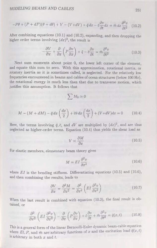
After combining équations (10.1) and (10.2), expanding, and then dropping the
higher order terms involving (dx)2, the resuit is
dV
d
dx
dx
_
dv
_ d2v
+ ~ q-Cdt~fhdt2
(10.3)
Next sum moments about point 0, the lower left corner of the element,
and equate this sum to zéro. With this approximation, rotational inertia, or
rotatory inertia as it is sometimes called, is neglected. For the relatively low
frequencies encountered in beams and cables of océan structures (below 100 Hz),
the rotational energy is much less than that due to transverse motion, which
justifies this assumption. It follows that
£Afo~0
M-(M + dM) - qdx (
j + cv dx I y j + (V+dV)dx = 0
(10.4)
Here, the terms involving q,c, and dV are multiplied by (dx)2, and are thus
neglected as higher-order terms. Equation (10.4) thus yields the shear load as
dM
dx
(10.5)
For elastic members, elementary beam theory gives
M = El—(10-6)
dx2
where El is the bending stiffness. Differentiating équations (10.5) and (10.6),
and then combining the results, leads to
dV_â^M_d^/ d^v\
(10.7)
dx “ dx2
dx2 \ dx2)
V
When the last resuit is combined with équation (10.3), the final resuit is obtained, or
(Pd /\+- cd ^+Æ=q(x,t)
(10.8)
dx2 y
dx2 )
dx \ dx )
dt
dt
This is a general form of the linear Bernoulli-Euler dynamic beam-cable équation
where El, P, and m are arbitrary functions of x and the excitation load q(x, t)
is arbitrary in both x and t.
251
-P0 + (P + dP)(0 + dff)+ V - (V+dV) + qdx - c^dx = mdx*— (10 2)
m
dt2
After combining équations (10.1) and (10.2), expanding, and then dropping the
higher order terms involving (dx)2, the resuit is
dV
d
dx
dx
_
dv
_ d2v
+ ~ q-Cdt~fhdt2
(10.3)
Next sum moments about point 0, the lower left corner of the element,
and equate this sum to zéro. With this approximation, rotational inertia, or
rotatory inertia as it is sometimes called, is neglected. For the relatively low
frequencies encountered in beams and cables of océan structures (below 100 Hz),
the rotational energy is much less than that due to transverse motion, which
justifies this assumption. It follows that
£Afo~0
M-(M + dM) - qdx (
j + cv dx I y j + (V+dV)dx = 0
(10.4)
Here, the terms involving q,c, and dV are multiplied by (dx)2, and are thus
neglected as higher-order terms. Equation (10.4) thus yields the shear load as
dM
dx
(10.5)
For elastic members, elementary beam theory gives
M = El—(10-6)
dx2
where El is the bending stiffness. Differentiating équations (10.5) and (10.6),
and then combining the results, leads to
dV_â^M_d^/ d^v\
(10.7)
dx “ dx2
dx2 \ dx2)
V
When the last resuit is combined with équation (10.3), the final resuit is obtained, or
(Pd /\+- cd ^+Æ=q(x,t)
(10.8)
dx2 y
dx2 )
dx \ dx )
dt
dt
This is a general form of the linear Bernoulli-Euler dynamic beam-cable équation
where El, P, and m are arbitrary functions of x and the excitation load q(x, t)
is arbitrary in both x and t.