

250
CONTINUOUS SYSTEMS
10.1 MODELING BEAMS AND CABLES
Governing Equations
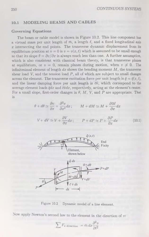
The beam or cable model is shown in Figure 10.2. This line component has
a virtual mass per unit length of m, a length £, and a fixed longitudinal axis
x intersecting the end points. The transverse dynamic displacement from its
equilibrium position at v = 0 is v = v(x, t) which is assumed to be small enough
so that its slope 6 = dv/dx is always much less than one. A further assumption,
which is also consistent with classical beam theory, is that transverse planes
at equilibrium, or v = 0, remain planes during motion, when v ■ 0. The
infinitésimal element of length dx shows the bending moment M, the transverse
shear load V, and the tension load P, ail of which are subject to small changes
across the element. The transverse excitation force per unit length is q ~ q(x, t),
and the linear damping force per unit length is cv, which correspond to the
average element loads qdx and cvdx, respectively, acting at the element’s center.
For a small slope, first-order changes in 6, M, V, and P are appropriate. That
is
/i jn
j
0 + d0 ~ — + -^~izdx ;
dx
dxz
,,
,»,
», cM/ ,
M + dA'I ~ M + ~7—dx
dx
dV
V+
V+ — dxdx
dP
P + dP~P + -^-dx
dx
(10-1)
Figure 10.2 Dynamic model of a line element.
Now apply Newton s second law to the element in the direction of v:
Vf
_ - z? q2v
/ . ‘v direction — mtlT--—
dtz
CONTINUOUS SYSTEMS
10.1 MODELING BEAMS AND CABLES
Governing Equations
The beam or cable model is shown in Figure 10.2. This line component has
a virtual mass per unit length of m, a length £, and a fixed longitudinal axis
x intersecting the end points. The transverse dynamic displacement from its
equilibrium position at v = 0 is v = v(x, t) which is assumed to be small enough
so that its slope 6 = dv/dx is always much less than one. A further assumption,
which is also consistent with classical beam theory, is that transverse planes
at equilibrium, or v = 0, remain planes during motion, when v ■ 0. The
infinitésimal element of length dx shows the bending moment M, the transverse
shear load V, and the tension load P, ail of which are subject to small changes
across the element. The transverse excitation force per unit length is q ~ q(x, t),
and the linear damping force per unit length is cv, which correspond to the
average element loads qdx and cvdx, respectively, acting at the element’s center.
For a small slope, first-order changes in 6, M, V, and P are appropriate. That
is
/i jn
j
0 + d0 ~ — + -^~izdx ;
dx
dxz
,,
,»,
», cM/ ,
M + dA'I ~ M + ~7—dx
dx
dV
V+
V+ — dxdx
dP
P + dP~P + -^-dx
dx
(10-1)
Figure 10.2 Dynamic model of a line element.
Now apply Newton s second law to the element in the direction of v:
Vf
_ - z? q2v
/ . ‘v direction — mtlT--—
dtz