

232
APPLICATIONS OF MULTI-DEGREE OF FREEDOM ANALYSIS
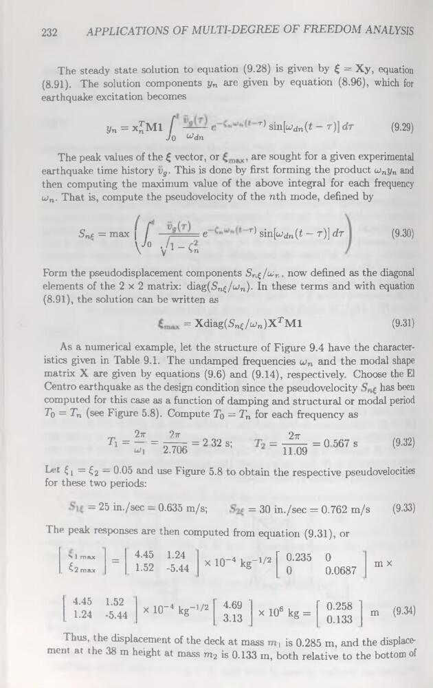
The steady State solution to équation (9.28) is given by £ = Xy, équation
(8.91). The solution components y„ are given by équation (8.96), which for
earthquake excitation becomes
yn = xjMl [
r) sm[u>dn(t - r)]dr
Jo udn
(9.29)
The peak values of the < vector, or
are sought for a given experimental
earthquake time history vg. This is done by first forming the product ujnyn and
then computing the maximum value of the above intégral for each frequency
ujn. That is, compute the pseudovelocity of the nth mode, defined by
Sne = max
( [
e
t) sin[wdn(t - r)] dr
\Jo . A _
\
V ‘ Sn
(9.30)
Form the pseudodisplacement components Sr^/ur.. now defined as the diagonal
éléments of the 2x2 matrix: diag(Sn^/un). In these terms and with équation
(8.91), the solution can be written as
= Xdiag(Snï/u,n)XTMl
(9.31)
As a numerical example, let the structure of Figure 9.4 hâve the characteristics given in Table 9.1. The undamped frequencies wn and the modal shape
matrix X are given by équations (9.6) and (9.14), respectively. Choose the El
Centro earthquake as the design condition since the pseudovelocity
has been
computed for this case as a function of damping and structural or modal period
7b = Tn (see Figure 5.8). Compute To = Tn for each frequency as
2tt
2ir
2tt
T, = ^=ÏSë = 2 32s;
= ïüœ =0567 !
M
L*'1 €1 = €2 — 0-05 and use Figure 5.8 to obtain the respective pseudovelocities
for these two periods:
— 25 in./sec — 0.635 m/s;
= 30 in./sec = 0.762 m/s
(9-33)
The peak responses are then computed from équation (9.31), or
s 1 max
. ^2 max
= 4.45 1.24
1.52 -5.44
X 10-4 kg -1/2 ' 0.235
0
0
0.0687
m x
4.45
. L24
1.52
-5.44
x 10-4 kg"’/2 4.69 '
3.13
x 106 kg =
‘ 0.258 '
0.133
m (9.34)
Thus, the displacement of the deck at mass m, is 0.285 m, and the displacement at the 38 m height at mass m2 is 0.133 m, both relative to the bottom of
APPLICATIONS OF MULTI-DEGREE OF FREEDOM ANALYSIS
The steady State solution to équation (9.28) is given by £ = Xy, équation
(8.91). The solution components y„ are given by équation (8.96), which for
earthquake excitation becomes
yn = xjMl [
r) sm[u>dn(t - r)]dr
Jo udn
(9.29)
The peak values of the < vector, or
are sought for a given experimental
earthquake time history vg. This is done by first forming the product ujnyn and
then computing the maximum value of the above intégral for each frequency
ujn. That is, compute the pseudovelocity of the nth mode, defined by
Sne = max
( [
e
t) sin[wdn(t - r)] dr
\Jo . A _
\
V ‘ Sn
(9.30)
Form the pseudodisplacement components Sr^/ur.. now defined as the diagonal
éléments of the 2x2 matrix: diag(Sn^/un). In these terms and with équation
(8.91), the solution can be written as
= Xdiag(Snï/u,n)XTMl
(9.31)
As a numerical example, let the structure of Figure 9.4 hâve the characteristics given in Table 9.1. The undamped frequencies wn and the modal shape
matrix X are given by équations (9.6) and (9.14), respectively. Choose the El
Centro earthquake as the design condition since the pseudovelocity
has been
computed for this case as a function of damping and structural or modal period
7b = Tn (see Figure 5.8). Compute To = Tn for each frequency as
2tt
2ir
2tt
T, = ^=ÏSë = 2 32s;
= ïüœ =0567 !
M
L*'1 €1 = €2 — 0-05 and use Figure 5.8 to obtain the respective pseudovelocities
for these two periods:
— 25 in./sec — 0.635 m/s;
= 30 in./sec = 0.762 m/s
(9-33)
The peak responses are then computed from équation (9.31), or
s 1 max
. ^2 max
= 4.45 1.24
1.52 -5.44
X 10-4 kg -1/2 ' 0.235
0
0
0.0687
m x
4.45
. L24
1.52
-5.44
x 10-4 kg"’/2 4.69 '
3.13
x 106 kg =
‘ 0.258 '
0.133
m (9.34)
Thus, the displacement of the deck at mass m, is 0.285 m, and the displacement at the 38 m height at mass m2 is 0.133 m, both relative to the bottom of