

A FIXED LEG PLATFORM
231
(9-20) as before. Computations showed that the response curves were nearly
identical to those of Figure 9.3, and that the absolute values of the first peaks
were:
klImax = 0 1937 m;
I€2|max = 0.0805 m
(9.26)
For this problem, then, linear wave theory is adéquate for preliminary dynamic
design.
Response to Earthquake Excitation
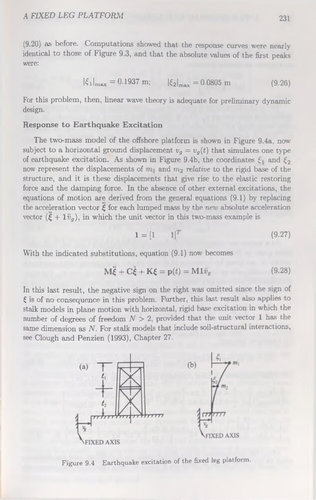
The two-mass model of the offshore platform is shown in Figure 9.4a, now
subject to a horizontal ground displacement vg = vg(t) that simulâtes one type
of earthquake excitation. As shown in Figure 9.4b, the coordinates ; and
now represent the displacements of
and m? relative to the rigid base of the
structure, and it is these displacements that give rise to the elastic restoring
force and the damping force. In the absence of other external excitations, the
équations of motion are derived from the general équations (9.1) by replacing
the accélération vector £ for each lumped mass by the new absolute accélération
vector (£ + liiff), in which the unit vector in this two-mass example is
1 = [1
With the indicated substitutions, équation (9.1) now becomes
M£ + C$ + K£ = p(i) = Mlvtf
(9.27)
(9.28)
In this last resuit, the négative sign on the right was omitted since the sign of
£ is of no conséquence in this problem. Further, this last resuit also applies to
stalk models in plane motion with horizontal, rigid base excitation in which the
number of degrees of freedom N > 2, provided that the unit vector 1 has the
same dimension as N. For stalk models that include soil-structural interactions,
see Clough and Penzien (1993), Chapter 27.
Figure 9.4 Earthquake excitation of the fixed leg platform.
231
(9-20) as before. Computations showed that the response curves were nearly
identical to those of Figure 9.3, and that the absolute values of the first peaks
were:
klImax = 0 1937 m;
I€2|max = 0.0805 m
(9.26)
For this problem, then, linear wave theory is adéquate for preliminary dynamic
design.
Response to Earthquake Excitation
The two-mass model of the offshore platform is shown in Figure 9.4a, now
subject to a horizontal ground displacement vg = vg(t) that simulâtes one type
of earthquake excitation. As shown in Figure 9.4b, the coordinates ; and
now represent the displacements of
and m? relative to the rigid base of the
structure, and it is these displacements that give rise to the elastic restoring
force and the damping force. In the absence of other external excitations, the
équations of motion are derived from the general équations (9.1) by replacing
the accélération vector £ for each lumped mass by the new absolute accélération
vector (£ + liiff), in which the unit vector in this two-mass example is
1 = [1
With the indicated substitutions, équation (9.1) now becomes
M£ + C$ + K£ = p(i) = Mlvtf
(9.27)
(9.28)
In this last resuit, the négative sign on the right was omitted since the sign of
£ is of no conséquence in this problem. Further, this last resuit also applies to
stalk models in plane motion with horizontal, rigid base excitation in which the
number of degrees of freedom N > 2, provided that the unit vector 1 has the
same dimension as N. For stalk models that include soil-structural interactions,
see Clough and Penzien (1993), Chapter 27.
Figure 9.4 Earthquake excitation of the fixed leg platform.