

218
MULTI-DEGREE OF FREEDOM LINEAR STRUCTURES
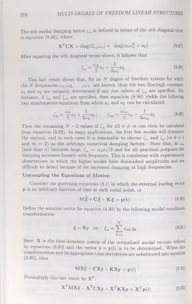
The nth modal damping factor
XrCX = diag(2(nun) = diag(aiw?, + a2)
(8.87)
After equating the nth diagonal terms above, it follows that
C„ = y «i +
(8.88)
This last resuit shows that, for an N degree of freedom System for which
the N frequencies w1,W2, ■ • ■ .~’.v are known, then the two Rayleigh constants
ai and a2 are uniquely determined if any two values of
are specified. For
instance, if Çk and
are specified, then équation (8.88) yields the following
two simultaneous équations from which «i and a2 can be calculated:
Qk = ^ai + xya2 ;
= y «1 +
(8'89)
Then the remaining N — 2 values of
for ail n / m can then be calculated
from équation (8.88). In many applications, the first few modes will dominate
the motion, and in such cases it is reasonable to choose , and Cj (or fc = 1
and m = 2) as the arbitrary numerical damping factors. Note that, as un
(and thus n) becomes large, Qn —» wnai/2 and for ail practical purposes the
damping increases linearly with frequency. This is consistent with experimental
observations in which the higher modes hâve diminished amplitudes and are
difficult to detect because of the increased damping at high frequencies.
Uncoupling the Equations of Motion
Consider the governing équations (8.1) in which the external loading vector
p is an arbitrary function of time at each nodal point, or
MÉ + C£ + K£ = p(t)
(8.90)
Define the solution vector for équation (8.90) by the following modal coordinate
transformation:
£ = Xy or Çn = ^xnkyk
(8.91)
fc=i
Here, X is the time-invariant matrix of the normalized modal vectors defined
by équations (8.80) and the vector y = y(t) is to be determined. When this
t ransformation and its appropriate time dérivatives are substituted into équation
(8.90), then
MXÿ + CXÿ + KXy = p(t)
(8-92)
Premultiply this last resuit by XT:
X ' MXÿ 1 XrCXÿ + XTKXy = xjîp(t)
(8-93)
MULTI-DEGREE OF FREEDOM LINEAR STRUCTURES
The nth modal damping factor
XrCX = diag(2(nun) = diag(aiw?, + a2)
(8.87)
After equating the nth diagonal terms above, it follows that
C„ = y «i +
(8.88)
This last resuit shows that, for an N degree of freedom System for which
the N frequencies w1,W2, ■ • ■ .~’.v are known, then the two Rayleigh constants
ai and a2 are uniquely determined if any two values of
are specified. For
instance, if Çk and
are specified, then équation (8.88) yields the following
two simultaneous équations from which «i and a2 can be calculated:
Qk = ^ai + xya2 ;
= y «1 +
(8'89)
Then the remaining N — 2 values of
for ail n / m can then be calculated
from équation (8.88). In many applications, the first few modes will dominate
the motion, and in such cases it is reasonable to choose , and Cj (or fc = 1
and m = 2) as the arbitrary numerical damping factors. Note that, as un
(and thus n) becomes large, Qn —» wnai/2 and for ail practical purposes the
damping increases linearly with frequency. This is consistent with experimental
observations in which the higher modes hâve diminished amplitudes and are
difficult to detect because of the increased damping at high frequencies.
Uncoupling the Equations of Motion
Consider the governing équations (8.1) in which the external loading vector
p is an arbitrary function of time at each nodal point, or
MÉ + C£ + K£ = p(t)
(8.90)
Define the solution vector for équation (8.90) by the following modal coordinate
transformation:
£ = Xy or Çn = ^xnkyk
(8.91)
fc=i
Here, X is the time-invariant matrix of the normalized modal vectors defined
by équations (8.80) and the vector y = y(t) is to be determined. When this
t ransformation and its appropriate time dérivatives are substituted into équation
(8.90), then
MXÿ + CXÿ + KXy = p(t)
(8-92)
Premultiply this last resuit by XT:
X ' MXÿ 1 XrCXÿ + XTKXy = xjîp(t)
(8-93)