

SUMMARY OF THE NORMAL MODE METHOD
219
In this last équation, it is noted that the coefficients of ÿ, ÿ, and y are defined
by équations (8.82), (8.87), and (8.83), respectively, which leads to
ÿ + diag(2(ncj„)ÿ + diag(u£)y _ Xrp(t)
(8.94)
These transformed équations (8.94) are observed to be uncoupled. The équation
for the nth mode is thus
ÿn + 2(nun^ +uj2ÿn = x^p(t)
(8.95)
Note that the right side of the last équation is a scalar quantity.
Steady State Solutions
It is recognized that the scalar équation (8.95) is in the form of the single
degree of freedom model, équation (5.58). The steady State Duhamel intégral
solution, équation (5.56), was derived for the latter model in Chapter 5. For the
présent case, this intégral solution can be derived in the same way. The resuit
is
ynXnP T
T)sin[u\in(t - r)]dr
JO
^dn
(8.96)
where the damped frequency for the nth mode is
(8.97)
The vector y expressed in terms of its components computed from équation
(8.96) is
y = [î/i,y2,.- • ,vn]t
(8.98)
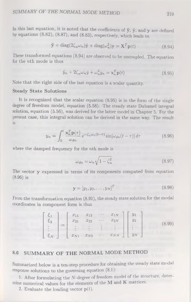
From the transformation équation (8.91), the steady State solution for the modal
coordinates in component form is thus
—
—
*11
*12
• •
*1/V
y\
€2
*21
*22
•
*2N
y?
*N1
*/V2
‘ •
*2V.V
. yN
(8.99)
8 6 SUMMARY OF THE NORMAL MODE METHOD
Summarized below is a ten-step procedure for obtaining the steady state modal
response solutions to the governing équation (8.1):
1. After formulating the 7V-degree of freedom model of the structure, détermine numerical values for the éléments of the M and K matrices.
2.
Evaluate the loading vector p(t).
219
In this last équation, it is noted that the coefficients of ÿ, ÿ, and y are defined
by équations (8.82), (8.87), and (8.83), respectively, which leads to
ÿ + diag(2(ncj„)ÿ + diag(u£)y _ Xrp(t)
(8.94)
These transformed équations (8.94) are observed to be uncoupled. The équation
for the nth mode is thus
ÿn + 2(nun^ +uj2ÿn = x^p(t)
(8.95)
Note that the right side of the last équation is a scalar quantity.
Steady State Solutions
It is recognized that the scalar équation (8.95) is in the form of the single
degree of freedom model, équation (5.58). The steady State Duhamel intégral
solution, équation (5.56), was derived for the latter model in Chapter 5. For the
présent case, this intégral solution can be derived in the same way. The resuit
is
ynXnP T
T)sin[u\in(t - r)]dr
JO
^dn
(8.96)
where the damped frequency for the nth mode is
(8.97)
The vector y expressed in terms of its components computed from équation
(8.96) is
y = [î/i,y2,.- • ,vn]t
(8.98)
From the transformation équation (8.91), the steady State solution for the modal
coordinates in component form is thus
—
—
*11
*12
• •
*1/V
y\
€2
*21
*22
•
*2N
y?
*N1
*/V2
‘ •
*2V.V
. yN
(8.99)
8 6 SUMMARY OF THE NORMAL MODE METHOD
Summarized below is a ten-step procedure for obtaining the steady state modal
response solutions to the governing équation (8.1):
1. After formulating the 7V-degree of freedom model of the structure, détermine numerical values for the éléments of the M and K matrices.
2.
Evaluate the loading vector p(t).