

382
Chemical Oceanography, 4th Edition
(b) aerosol scattering, and (c) the diffuse transmittance of the atmosphere, all of which
must be computed to propagate the signal leaving the water and reaching the level of the
satellite. Once these corrections are made, one can estimate the water leaving radiance.
Bio- optic algorithms must be used to calculate the relevant quantities, such as chlorophyll
and primary production. This must be done by correction for the optical properties of the
surface waters. This is normally done using empirical equations that attempt to link the
upwelling radiance Lw and the concentration of pigments (Gordon et al., 1988):
C = 1.15 (Lw(443)/Lw(569) –1.42 , C < 1 mg m –3 (Green water)
C = 3.64 (Lw(500)/Lw(560) –2.62 , C < 1 mg m –3 (Blue water)
The occurrence of blooms of phytoplankton with shells of CaCO 3 can lead to high reflectance because of the milky waters (Balch et al., 1993). The calculation of the integrative
total productivity uses complicated equations that depend on the surface irradiance and
parameters related to bio- optical properties of the waters. The estimation of new production and the carbon flux across the air–sea interface are more difficult to determine. As
more global data become available, these parameterizations will be improved.
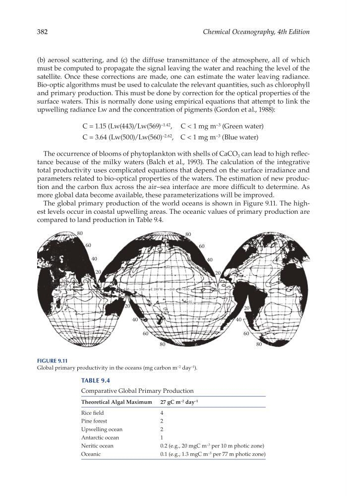
The global primary production of the world oceans is shown in Figure 9.11. The highest levels occur in coastal upwelling areas. The oceanic values of primary production are
compared to land production in Table 9.4.
20
20
20
40
40
60
60
80
80
35
35
40
60
80
20
40
60
80
20 0
200
60
120
140
140
100
0 E
160
160
E 180 W
Figure 9.11
Global primary productivity in the oceans (mg carbon m –2 day –1 ).
Table 9.4
Comparative Global Primary Production
Theoretical Algal Maximum 27 gC m –2 day –1
Rice field
4
Pine forest
2
Upwelling ocean
2
Antarctic ocean
1
Neritic ocean
0.2 (e.g., 20 mgC m –3 per 10 m photic zone)
Oceanic
0.1 (e.g., 1.3 mgC m –3 per 77 m photic zone)
Chemical Oceanography, 4th Edition
(b) aerosol scattering, and (c) the diffuse transmittance of the atmosphere, all of which
must be computed to propagate the signal leaving the water and reaching the level of the
satellite. Once these corrections are made, one can estimate the water leaving radiance.
Bio- optic algorithms must be used to calculate the relevant quantities, such as chlorophyll
and primary production. This must be done by correction for the optical properties of the
surface waters. This is normally done using empirical equations that attempt to link the
upwelling radiance Lw and the concentration of pigments (Gordon et al., 1988):
C = 1.15 (Lw(443)/Lw(569) –1.42 , C < 1 mg m –3 (Green water)
C = 3.64 (Lw(500)/Lw(560) –2.62 , C < 1 mg m –3 (Blue water)
The occurrence of blooms of phytoplankton with shells of CaCO 3 can lead to high reflectance because of the milky waters (Balch et al., 1993). The calculation of the integrative
total productivity uses complicated equations that depend on the surface irradiance and
parameters related to bio- optical properties of the waters. The estimation of new production and the carbon flux across the air–sea interface are more difficult to determine. As
more global data become available, these parameterizations will be improved.
The global primary production of the world oceans is shown in Figure 9.11. The highest levels occur in coastal upwelling areas. The oceanic values of primary production are
compared to land production in Table 9.4.
20
20
20
40
40
60
60
80
80
35
35
40
60
80
20
40
60
80
20 0
200
60
120
140
140
100
0 E
160
160
E 180 W
Figure 9.11
Global primary productivity in the oceans (mg carbon m –2 day –1 ).
Table 9.4
Comparative Global Primary Production
Theoretical Algal Maximum 27 gC m –2 day –1
Rice field
4
Pine forest
2
Upwelling ocean
2
Antarctic ocean
1
Neritic ocean
0.2 (e.g., 20 mgC m –3 per 10 m photic zone)
Oceanic
0.1 (e.g., 1.3 mgC m –3 per 77 m photic zone)