

a dual assimilation approach utilizing the model’s
adjoint and an approximate Kalman filter and
smoother. The forward component is the general
circulation model described in Marshall et al.
(1997a,b). The adjoint component is obtained from
the forward model by using the Tangent-linear and
Adjoint Compiler of Giering and Kaminski,
(1998). This compiler has proven to be extremely
flexible since it allows one to easily regenerate the
adjoint code whenever a change in the forward
code is necessary (Marotzke et al., 1999). The
approximate filter is an extension of the reducedstate filter described by Fukumori and MalanotteRizzoli (1995).
Ongoing computations include a 6-year estimate
of the time-evolving ocean circulation (1992
through 1997) with up to 1° spatial resolution, a
complete mixed-layer model (Large et al., 1994) and
an eddy parameterization (Gent and McWilliams,
1990). Data include the absolute and time-varying
T/P data from October 1992 through December
1997, SSH anomalies from the ERS-1 and ERS-2
satellites, monthly mean SST data (Reynolds and
Smith, 1994), time-varying NCEP re-analysis fluxes
of momentum, heat and fresh water, and NSCAT
estimates of wind stress errors. Monthly means of
the model state are required to remain within
assigned bounds of the monthly mean Levitus
et al. (1994b) climatology. To bring the model
into consistency with the observations, the initial
potential temperature () and salinity (S) fields are
modified, as well as the surface forcing fields.
Changes in those fields (often referred to as
‘control’ terms) are determined as a best-fit in a
least-squares sense of the model state to the observations and their uncertainties over the full data
period. In the current configuration, there are
10
8
–10
9 elements in the control vector.
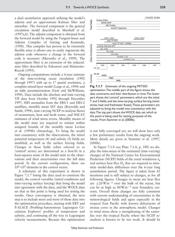
A schematic of this experiment is shown in
Figure 7.1.7 listing the data used to constrain the
model, the control variables (initial conditions and
time-varying surface forcing) that bring the model
into agreement with the data, and the WOCE data
set that at this point is being used for testing the
results. Once convergence is obtained, the next
step is to include more and more of those data into
the optimization procedure, starting with XBT and
P-ALACE (Profiling-Autonomous Lagrangian Circulation Explorer) profiles of temperature and
salinity, and continuing all the way to Lagrangian
velocity measurements. Because this optimization
is not fully converged yet, we will show here only
a few preliminary results from the ongoing work.
More details are given in Stammer et al. (1997,
2000b).
In Figure 7.1.8 (see Plate 7.1.8, p. 588) we display the time-mean of the estimated (time-varying)
changes of the National Center for Environmental
Prediction (NCEP) fields of the zonal windstress x
and surface heat flux H q that are required to minimize model-data differences over the 6-year long
assimilation period. The figure is taken from 43
iterations and is still subject to changes, as for all
following figures. Changes in mean net heat flux
are <20 W m
92 over the bulk of the ocean, but
can be as high as 80 W m
92 near boundary currents. Overall those changes are fully consistent
with current understanding of uncertainties in the
meteorological fields and agree especially in the
tropical East Pacific with known deficiencies of
stratus cover in the atmospheric model. Changes
in wind stress show a strengthening of the easterlies over the tropical Pacific where the NCEP reanalysis is known to be too weak. It should be
7.1 Towards a WOCE Synthesis
539
Talley, Stammer and Fukumori
ERS-2 SSH'
ERS-1 SSH'
T0, S0
tau(t)
Hq(t)
Hs(t)
Test Data
Controls
Data Constraints
U0, V0
1992
1993
1994
1995
1996
1997
Profiles
P-ALACE
Surface Drifter
WOCE WHP
ALACE Trajectories
XBT Profiles
monthly Reynolds SST
mean TP SSH - EGM96
daily TP SSH'
tau_ncep
Hq_ncep
Hs_ncep
T_lev
monthly
S_lev
monthly
Fig. 7.1.7 Schematic of the ongoing MIT/SIO
optimization.The middle part of the figure shows the
data constraints and their distribution in time.The lower
part shows the ‘control’ parameters, which are the initial
T and S fields, and the time-varying surface forcing (wind
stress, heat and freshwater fluxes).Those parameters are
adjusted to bring the model into consistency with the
data.The top part shows the WOCE data set, which at
this point is being used for testing purposes of the
results. From Stammer et al. (2000b).
adjoint and an approximate Kalman filter and
smoother. The forward component is the general
circulation model described in Marshall et al.
(1997a,b). The adjoint component is obtained from
the forward model by using the Tangent-linear and
Adjoint Compiler of Giering and Kaminski,
(1998). This compiler has proven to be extremely
flexible since it allows one to easily regenerate the
adjoint code whenever a change in the forward
code is necessary (Marotzke et al., 1999). The
approximate filter is an extension of the reducedstate filter described by Fukumori and MalanotteRizzoli (1995).
Ongoing computations include a 6-year estimate
of the time-evolving ocean circulation (1992
through 1997) with up to 1° spatial resolution, a
complete mixed-layer model (Large et al., 1994) and
an eddy parameterization (Gent and McWilliams,
1990). Data include the absolute and time-varying
T/P data from October 1992 through December
1997, SSH anomalies from the ERS-1 and ERS-2
satellites, monthly mean SST data (Reynolds and
Smith, 1994), time-varying NCEP re-analysis fluxes
of momentum, heat and fresh water, and NSCAT
estimates of wind stress errors. Monthly means of
the model state are required to remain within
assigned bounds of the monthly mean Levitus
et al. (1994b) climatology. To bring the model
into consistency with the observations, the initial
potential temperature () and salinity (S) fields are
modified, as well as the surface forcing fields.
Changes in those fields (often referred to as
‘control’ terms) are determined as a best-fit in a
least-squares sense of the model state to the observations and their uncertainties over the full data
period. In the current configuration, there are
10
8
–10
9 elements in the control vector.
A schematic of this experiment is shown in
Figure 7.1.7 listing the data used to constrain the
model, the control variables (initial conditions and
time-varying surface forcing) that bring the model
into agreement with the data, and the WOCE data
set that at this point is being used for testing the
results. Once convergence is obtained, the next
step is to include more and more of those data into
the optimization procedure, starting with XBT and
P-ALACE (Profiling-Autonomous Lagrangian Circulation Explorer) profiles of temperature and
salinity, and continuing all the way to Lagrangian
velocity measurements. Because this optimization
is not fully converged yet, we will show here only
a few preliminary results from the ongoing work.
More details are given in Stammer et al. (1997,
2000b).
In Figure 7.1.8 (see Plate 7.1.8, p. 588) we display the time-mean of the estimated (time-varying)
changes of the National Center for Environmental
Prediction (NCEP) fields of the zonal windstress x
and surface heat flux H q that are required to minimize model-data differences over the 6-year long
assimilation period. The figure is taken from 43
iterations and is still subject to changes, as for all
following figures. Changes in mean net heat flux
are <20 W m
92 over the bulk of the ocean, but
can be as high as 80 W m
92 near boundary currents. Overall those changes are fully consistent
with current understanding of uncertainties in the
meteorological fields and agree especially in the
tropical East Pacific with known deficiencies of
stratus cover in the atmospheric model. Changes
in wind stress show a strengthening of the easterlies over the tropical Pacific where the NCEP reanalysis is known to be too weak. It should be
7.1 Towards a WOCE Synthesis
539
Talley, Stammer and Fukumori
ERS-2 SSH'
ERS-1 SSH'
T0, S0
tau(t)
Hq(t)
Hs(t)
Test Data
Controls
Data Constraints
U0, V0
1992
1993
1994
1995
1996
1997
Profiles
P-ALACE
Surface Drifter
WOCE WHP
ALACE Trajectories
XBT Profiles
monthly Reynolds SST
mean TP SSH - EGM96
daily TP SSH'
tau_ncep
Hq_ncep
Hs_ncep
T_lev
monthly
S_lev
monthly
Fig. 7.1.7 Schematic of the ongoing MIT/SIO
optimization.The middle part of the figure shows the
data constraints and their distribution in time.The lower
part shows the ‘control’ parameters, which are the initial
T and S fields, and the time-varying surface forcing (wind
stress, heat and freshwater fluxes).Those parameters are
adjusted to bring the model into consistency with the
data.The top part shows the WOCE data set, which at
this point is being used for testing purposes of the
results. From Stammer et al. (2000b).