

noted that the small-scale features in the wind
stress changes arise to some extent from the lack
of a full wind stress error covariance function in the
current optimization. The displayed changes and
similar changes in meridional wind stress and fresh
water flux will be used to understand and improve
uncertainties in meteorological forcing fields after a
fully optimized solution has been obtained.
Estimated mean fields of sea surface height and
the near-surface flow field and the flow and temperature fields at 610 and 2450 m depth are shown
in Figures 7.1.9 (see Plate 7.1.9, p. 588). All major
ocean current structures are well represented and
the largest deficiency – the lack of small-scale
structures – can be primarily attributed to the still
coarse resolution of the optimization. (The figure
actually stems from iterations being performed on
a 2° spatial resolution.)
The model–data misfit of absolute sea surface
height is displayed in Figure 7.1.10 (see Plate 7.1.10,
p. 588). Differences are as large as 40 cm, especially
in the Southern Ocean. There is a close correlation
of the residuals with independent information about
the error of the EGM96 geoid model over many
parts of the global ocean. The associated difference
between the first-guess mean flow field at 575 m
depth and that obtained from the constrained model
is shown in the lower panel of the figure. In many
events, changes in the large-scale current structure
are apparent with maximum amplitudes about
1.2 cm s
91
, or a full 30% of the mean.
An important climate-related issue is the question of the amount of heat the ocean carries and
how variable it is in time. To illustrate what can
be expected from the estimated fields for a WOCE
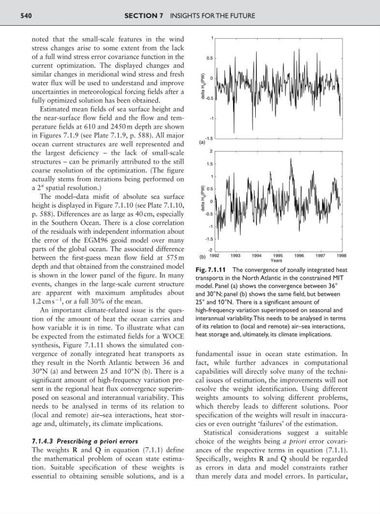
synthesis, Figure 7.1.11 shows the simulated convergence of zonally integrated heat transports as
they result in the North Atlantic between 36 and
30°N (a) and between 25 and 10°N (b). There is a
significant amount of high-frequency variation present in the regional heat flux convergence superimposed on seasonal and interannual variability. This
needs to be analysed in terms of its relation to
(local and remote) air–sea interactions, heat storage and, ultimately, its climate implications.
7.1.4.3 Prescribing a priori errors
The weights R and Q in equation (7.1.1) define
the mathematical problem of ocean state estimation. Suitable specification of these weights is
essential to obtaining sensible solutions, and is a
fundamental issue in ocean state estimation. In
fact, while further advances in computational
capabilities will directly solve many of the technical issues of estimation, the improvements will not
resolve the weight identification. Using different
weights amounts to solving different problems,
which thereby leads to different solutions. Poor
specification of the weights will result in inaccuracies or even outright ‘failures’ of the estimation.
Statistical considerations suggest a suitable
choice of the weights being a priori error covariances of the respective terms in equation (7.1.1).
Specifically, weights R and Q should be regarded
as errors in data and model constraints rather
than merely data and model errors. In particular,
SECTION 7 INSIGHTS FOR THE FUTURE
540
-1.5
-1
-0.5
0
0.5
1
delta H
q (PW)
delta H
q (PW)
1992
1993
1994
1995
1996
1997
1998
-2
-1.5
-1
-0.5
0
0.5
1
1.5
2
Years
(a)
(b)
Fig. 7.1.11 The convergence of zonally integrated heat
transports in the North Atlantic in the constrained MIT
model. Panel (a) shows the convergence between 36°
and 30°N; panel (b) shows the same field, but between
25° and 10°N. There is a significant amount of
high-frequency variation superimposed on seasonal and
interannual variability.This needs to be analysed in terms
of its relation to (local and remote) air–sea interactions,
heat storage and, ultimately, its climate implications.
stress changes arise to some extent from the lack
of a full wind stress error covariance function in the
current optimization. The displayed changes and
similar changes in meridional wind stress and fresh
water flux will be used to understand and improve
uncertainties in meteorological forcing fields after a
fully optimized solution has been obtained.
Estimated mean fields of sea surface height and
the near-surface flow field and the flow and temperature fields at 610 and 2450 m depth are shown
in Figures 7.1.9 (see Plate 7.1.9, p. 588). All major
ocean current structures are well represented and
the largest deficiency – the lack of small-scale
structures – can be primarily attributed to the still
coarse resolution of the optimization. (The figure
actually stems from iterations being performed on
a 2° spatial resolution.)
The model–data misfit of absolute sea surface
height is displayed in Figure 7.1.10 (see Plate 7.1.10,
p. 588). Differences are as large as 40 cm, especially
in the Southern Ocean. There is a close correlation
of the residuals with independent information about
the error of the EGM96 geoid model over many
parts of the global ocean. The associated difference
between the first-guess mean flow field at 575 m
depth and that obtained from the constrained model
is shown in the lower panel of the figure. In many
events, changes in the large-scale current structure
are apparent with maximum amplitudes about
1.2 cm s
91
, or a full 30% of the mean.
An important climate-related issue is the question of the amount of heat the ocean carries and
how variable it is in time. To illustrate what can
be expected from the estimated fields for a WOCE
synthesis, Figure 7.1.11 shows the simulated convergence of zonally integrated heat transports as
they result in the North Atlantic between 36 and
30°N (a) and between 25 and 10°N (b). There is a
significant amount of high-frequency variation present in the regional heat flux convergence superimposed on seasonal and interannual variability. This
needs to be analysed in terms of its relation to
(local and remote) air–sea interactions, heat storage and, ultimately, its climate implications.
7.1.4.3 Prescribing a priori errors
The weights R and Q in equation (7.1.1) define
the mathematical problem of ocean state estimation. Suitable specification of these weights is
essential to obtaining sensible solutions, and is a
fundamental issue in ocean state estimation. In
fact, while further advances in computational
capabilities will directly solve many of the technical issues of estimation, the improvements will not
resolve the weight identification. Using different
weights amounts to solving different problems,
which thereby leads to different solutions. Poor
specification of the weights will result in inaccuracies or even outright ‘failures’ of the estimation.
Statistical considerations suggest a suitable
choice of the weights being a priori error covariances of the respective terms in equation (7.1.1).
Specifically, weights R and Q should be regarded
as errors in data and model constraints rather
than merely data and model errors. In particular,
SECTION 7 INSIGHTS FOR THE FUTURE
540
-1.5
-1
-0.5
0
0.5
1
delta H
q (PW)
delta H
q (PW)
1992
1993
1994
1995
1996
1997
1998
-2
-1.5
-1
-0.5
0
0.5
1
1.5
2
Years
(a)
(b)
Fig. 7.1.11 The convergence of zonally integrated heat
transports in the North Atlantic in the constrained MIT
model. Panel (a) shows the convergence between 36°
and 30°N; panel (b) shows the same field, but between
25° and 10°N. There is a significant amount of
high-frequency variation superimposed on seasonal and
interannual variability.This needs to be analysed in terms
of its relation to (local and remote) air–sea interactions,
heat storage and, ultimately, its climate implications.