

allows for explicitly accounting for uncertainties
in models and data, as well as evaluation of a
posteriori errors. However, because of significant
algorithmic and computational requirements in
implementing these optimal methods, many studies have explored alternate simpler approaches.
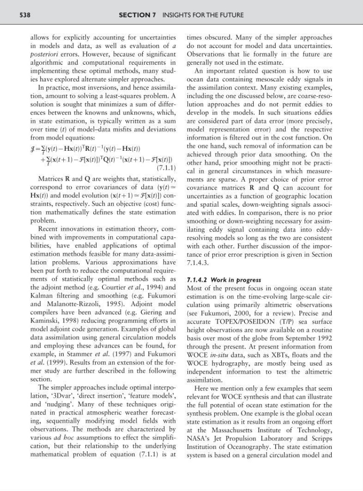
In practice, most inversions, and hence assimilation, amount to solving a least-squares problem. A
solution is sought that minimizes a sum of differences between the knowns and unknowns, which,
in state estimation, is typically written as a sum
over time (t) of model–data misfits and deviations
from model equations:
J:⌺
t
(y(t)9Hx(t))
T
R(t)
91
(y(t)9Hx(t))
;⌺
t
(x(t;1)9F[x(t)])
T
Q(t)
91
(x(t;1)9F[x(t)])
(7.1.1)
Matrices R and Q are weights that, statistically,
correspond to error covariances of data (y(t) Ӎ
Hx(t)) and model evolution (x(t;1) Ӎ F[x(t)]) constraints, respectively. Such an objective (cost) function mathematically defines the state estimation
problem.
Recent innovations in estimation theory, combined with improvements in computational capabilities, have enabled applications of optimal
estimation methods feasible for many data-assimilation problems. Various approximations have
been put forth to reduce the computational requirements of statistically optimal methods such as
the adjoint method (e.g. Courtier et al., 1994) and
Kalman filtering and smoothing (e.g. Fukumori
and Malanotte-Rizzoli, 1995). Adjoint model
compilers have been advanced (e.g. Giering and
Kaminski, 1998) reducing programming efforts in
model adjoint code generation. Examples of global
data assimilation using general circulation models
and employing these advances can be found, for
example, in Stammer et al. (1997) and Fukumori
et al. (1999). Results from an extension of the former study are further described in the following
section.
The simpler approaches include optimal interpolation, ‘3Dvar’, ‘direct insertion’, ‘feature models’,
and ‘nudging’. Many of these techniques originated in practical atmospheric weather forecasting, sequentially modifying model fields with
observations. The methods are characterized by
various ad hoc assumptions to effect the simplification, but their relationship to the underlying
mathematical problem of equation (7.1.1) is at
times obscured. Many of the simpler approaches
do not account for model and data uncertainties.
Observations that lie formally in the future are
generally not used in the estimate.
An important related question is how to use
ocean data containing mesoscale eddy signals in
the assimilation context. Many existing examples,
including the one discussed below, are coarse-resolution approaches and do not permit eddies to
develop in the models. In such situations eddies
are considered part of data error (more precisely,
model representation error) and the respective
information is filtered out in the cost function. On
the one hand, such removal of information can be
achieved through prior data smoothing. On the
other hand, prior smoothing might not be practical in general circumstances in which measurements are sparse. A proper choice of prior error
covariance matrices R and Q can account for
uncertainties as a function of geographic location
and spatial scales, down-weighting signals associated with eddies. In comparison, there is no prior
smoothing or down-weighting necessary for assimilating eddy signal containing data into eddyresolving models so long as the two are consistent
with each other. Further discussion of the importance of prior error prescription is given in Section
7.1.4.3.
7.1.4.2 Work in progress
Most of the present focus in ongoing ocean state
estimation is on the time-evolving large-scale circulation using primarily altimetric observations
(see Fukumori, 2000, for a review). Precise and
accurate TOPEX/POSEIDON (T/P) sea surface
height observations are now available on a routine
basis over most of the globe from September 1992
through the present. At present information from
WOCE in-situ data, such as XBTs, floats and the
WOCE hydrography, are mostly being used as
independent information to test the altimetric
assimilation.
Here we mention only a few examples that seem
relevant for WOCE synthesis and that can illustrate
the full potential of ocean state estimation for the
synthesis problem. One example is the global ocean
state estimation as it results from an ongoing effort
at the Massachusetts Institute of Technology,
NASA’s Jet Propulsion Laboratory and Scripps
Institution of Oceanography. The state estimation
system is based on a general circulation model and
SECTION 7 INSIGHTS FOR THE FUTURE
538
in models and data, as well as evaluation of a
posteriori errors. However, because of significant
algorithmic and computational requirements in
implementing these optimal methods, many studies have explored alternate simpler approaches.
In practice, most inversions, and hence assimilation, amount to solving a least-squares problem. A
solution is sought that minimizes a sum of differences between the knowns and unknowns, which,
in state estimation, is typically written as a sum
over time (t) of model–data misfits and deviations
from model equations:
J:⌺
t
(y(t)9Hx(t))
T
R(t)
91
(y(t)9Hx(t))
;⌺
t
(x(t;1)9F[x(t)])
T
Q(t)
91
(x(t;1)9F[x(t)])
(7.1.1)
Matrices R and Q are weights that, statistically,
correspond to error covariances of data (y(t) Ӎ
Hx(t)) and model evolution (x(t;1) Ӎ F[x(t)]) constraints, respectively. Such an objective (cost) function mathematically defines the state estimation
problem.
Recent innovations in estimation theory, combined with improvements in computational capabilities, have enabled applications of optimal
estimation methods feasible for many data-assimilation problems. Various approximations have
been put forth to reduce the computational requirements of statistically optimal methods such as
the adjoint method (e.g. Courtier et al., 1994) and
Kalman filtering and smoothing (e.g. Fukumori
and Malanotte-Rizzoli, 1995). Adjoint model
compilers have been advanced (e.g. Giering and
Kaminski, 1998) reducing programming efforts in
model adjoint code generation. Examples of global
data assimilation using general circulation models
and employing these advances can be found, for
example, in Stammer et al. (1997) and Fukumori
et al. (1999). Results from an extension of the former study are further described in the following
section.
The simpler approaches include optimal interpolation, ‘3Dvar’, ‘direct insertion’, ‘feature models’,
and ‘nudging’. Many of these techniques originated in practical atmospheric weather forecasting, sequentially modifying model fields with
observations. The methods are characterized by
various ad hoc assumptions to effect the simplification, but their relationship to the underlying
mathematical problem of equation (7.1.1) is at
times obscured. Many of the simpler approaches
do not account for model and data uncertainties.
Observations that lie formally in the future are
generally not used in the estimate.
An important related question is how to use
ocean data containing mesoscale eddy signals in
the assimilation context. Many existing examples,
including the one discussed below, are coarse-resolution approaches and do not permit eddies to
develop in the models. In such situations eddies
are considered part of data error (more precisely,
model representation error) and the respective
information is filtered out in the cost function. On
the one hand, such removal of information can be
achieved through prior data smoothing. On the
other hand, prior smoothing might not be practical in general circumstances in which measurements are sparse. A proper choice of prior error
covariance matrices R and Q can account for
uncertainties as a function of geographic location
and spatial scales, down-weighting signals associated with eddies. In comparison, there is no prior
smoothing or down-weighting necessary for assimilating eddy signal containing data into eddyresolving models so long as the two are consistent
with each other. Further discussion of the importance of prior error prescription is given in Section
7.1.4.3.
7.1.4.2 Work in progress
Most of the present focus in ongoing ocean state
estimation is on the time-evolving large-scale circulation using primarily altimetric observations
(see Fukumori, 2000, for a review). Precise and
accurate TOPEX/POSEIDON (T/P) sea surface
height observations are now available on a routine
basis over most of the globe from September 1992
through the present. At present information from
WOCE in-situ data, such as XBTs, floats and the
WOCE hydrography, are mostly being used as
independent information to test the altimetric
assimilation.
Here we mention only a few examples that seem
relevant for WOCE synthesis and that can illustrate
the full potential of ocean state estimation for the
synthesis problem. One example is the global ocean
state estimation as it results from an ongoing effort
at the Massachusetts Institute of Technology,
NASA’s Jet Propulsion Laboratory and Scripps
Institution of Oceanography. The state estimation
system is based on a general circulation model and
SECTION 7 INSIGHTS FOR THE FUTURE
538