

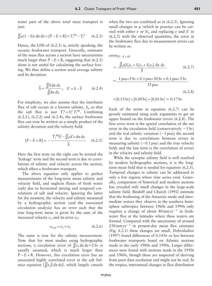
water part of the above total mass transport is
just:
͐͐(19S)v dx dz;[P9E;R]:T i
M
9T i
S
(6.2.3)
Hence, the LHS of (6.2.3) is, strictly speaking, the
oceanic freshwater transport. Generally, estimates
of the mass flux across a section have uncertainties
much larger than P9E;R, suggesting that (6.2.3)
alone is not useful for calculating the surface forcing. We thus define a section areal average salinity
and its deviation:
S
ෆ:
; SЈ:S9S ෆ
(6.2.4)
For simplicity, we also assume that the interbasin
flux of salt occurs at a known salinity, S i , so that
the salt flux is just T i
S
:S i
* T i
M . Combining
(6.2.1), (6.2.2) and (6.2.4), the surface freshwater
flux can now be written as a simple product of the
salinity deviation and the velocity field:
[P9E;R]:9
(6.2.5)
Here the first term on the right can be termed the
‘leakage’ term and the second term is due to correlations of salinity and velocity across the section,
which effect a freshwater transport.
The above equation only applies to perfect
measurements of the long-term mean salinity and
velocity field, and neglects fluxes of fresh water
(salt) due to horizontal mixing and temporal correlations of salt and velocity. Ignoring the latter
for the moment, the velocity and salinity measured
by a hydrographic section (and the associated
circulation analysis) has an error such that the
true long-term mean is given by the sum of the
measured velocity v o and its error v e :
v true :v o ;v e
(6.2.6)
The same is true for the salinity measurement.
Note that for most studies using hydrographic
sections, a circulation error of ͐͐v e dx dzϷ2 Sv is
usually assumed, which is much larger than
P9E;R. However, this circulation error has an
associated highly correlated error in the salt balance equation ( ͐͐ v e S ෆ dx dz), which largely cancels
when the two are combined as in (6.2.5). Ignoring
small changes in (which in practice can be carried with either v or S), and replacing v and SЈ in
(6.2.5) with the observed quantities, the error in
the freshwater flux due to measurement errors can
be written as:
error [P9E;R]
:
(6.2.7)
Ϸ
(6.2.8)
ϷͿ0.15 SvͿ;Ϳ0.09 SvͿ;Ϳ0.01 SvͿ Ϸ 0.17 Sv
Each of the terms in equation (6.2.7) can be
grossly estimated using scale arguments to get an
upper bound on the freshwater errors (6.2.8). The
first error term is the spatial correlation of the net
error in the circulation field (conservatively ϳ5 Sv)
and the real salinity variation (ϳ1 psu); the second
term is due to correlations between errors in
measuring salinity (ϳ0.1 psu) and the true velocity
field; and the last term is the correlation of errors
in the velocity and salinity field.
While the synoptic salinity field is well resolved
by modern hydrographic sections, it is the longterm mean field that is needed for equation (6.2.5).
Temporal changes in salinity can be addressed in
only a few regions where time series exist. Generally, comparison of historical and modern sections
has revealed only small changes in the large-scale
salinity field. Bindoff and Church (1992) estimate
that the freshening of the Antarctic mode and intermediate waters they observe in the southern hemisphere subtropics between 1960s and 1990s only
requires a change of about 40 mm yr
91 in freshwater flux at the latitudes where these waters are
formed. Compared with the uncertainty of around
250 mm yr
91 in present-day mean flux estimates
(Fig. 6.2.1) these changes are small. Dobroliubov
(1997) found differences of 0.14 Sv or less between
freshwater transports based on Atlantic sections
made in the early 1980s and 1990s. Larger differences were found with sections made in the 1950s
and 1960s, though these are suspected of deriving
from poor data resolution and might not be real. In
the tropics, interannual changes in flux distribution
1 psu * 5 Sv;0.1 psu * 30 Sv;0.1 psu * 5 Sv
ᎏᎏᎏᎏᎏ
35 psu
͐͐[SЈ o v e ;SЈ e v o ;SЈ e v e ] dx dz
ᎏᎏᎏᎏ
S ෆ
T i
M SЈ i 9͐͐SЈv dx dz
ᎏᎏᎏ
S ෆ
͐͐S dx dz
ᎏᎏ
͐͐dx dz
6.2 Ocean Transport of Fresh Water
481
Wijffels
just:
͐͐(19S)v dx dz;[P9E;R]:T i
M
9T i
S
(6.2.3)
Hence, the LHS of (6.2.3) is, strictly speaking, the
oceanic freshwater transport. Generally, estimates
of the mass flux across a section have uncertainties
much larger than P9E;R, suggesting that (6.2.3)
alone is not useful for calculating the surface forcing. We thus define a section areal average salinity
and its deviation:
S
ෆ:
; SЈ:S9S ෆ
(6.2.4)
For simplicity, we also assume that the interbasin
flux of salt occurs at a known salinity, S i , so that
the salt flux is just T i
S
:S i
* T i
M . Combining
(6.2.1), (6.2.2) and (6.2.4), the surface freshwater
flux can now be written as a simple product of the
salinity deviation and the velocity field:
[P9E;R]:9
(6.2.5)
Here the first term on the right can be termed the
‘leakage’ term and the second term is due to correlations of salinity and velocity across the section,
which effect a freshwater transport.
The above equation only applies to perfect
measurements of the long-term mean salinity and
velocity field, and neglects fluxes of fresh water
(salt) due to horizontal mixing and temporal correlations of salt and velocity. Ignoring the latter
for the moment, the velocity and salinity measured
by a hydrographic section (and the associated
circulation analysis) has an error such that the
true long-term mean is given by the sum of the
measured velocity v o and its error v e :
v true :v o ;v e
(6.2.6)
The same is true for the salinity measurement.
Note that for most studies using hydrographic
sections, a circulation error of ͐͐v e dx dzϷ2 Sv is
usually assumed, which is much larger than
P9E;R. However, this circulation error has an
associated highly correlated error in the salt balance equation ( ͐͐ v e S ෆ dx dz), which largely cancels
when the two are combined as in (6.2.5). Ignoring
small changes in (which in practice can be carried with either v or S), and replacing v and SЈ in
(6.2.5) with the observed quantities, the error in
the freshwater flux due to measurement errors can
be written as:
error [P9E;R]
:
(6.2.7)
Ϸ
(6.2.8)
ϷͿ0.15 SvͿ;Ϳ0.09 SvͿ;Ϳ0.01 SvͿ Ϸ 0.17 Sv
Each of the terms in equation (6.2.7) can be
grossly estimated using scale arguments to get an
upper bound on the freshwater errors (6.2.8). The
first error term is the spatial correlation of the net
error in the circulation field (conservatively ϳ5 Sv)
and the real salinity variation (ϳ1 psu); the second
term is due to correlations between errors in
measuring salinity (ϳ0.1 psu) and the true velocity
field; and the last term is the correlation of errors
in the velocity and salinity field.
While the synoptic salinity field is well resolved
by modern hydrographic sections, it is the longterm mean field that is needed for equation (6.2.5).
Temporal changes in salinity can be addressed in
only a few regions where time series exist. Generally, comparison of historical and modern sections
has revealed only small changes in the large-scale
salinity field. Bindoff and Church (1992) estimate
that the freshening of the Antarctic mode and intermediate waters they observe in the southern hemisphere subtropics between 1960s and 1990s only
requires a change of about 40 mm yr
91 in freshwater flux at the latitudes where these waters are
formed. Compared with the uncertainty of around
250 mm yr
91 in present-day mean flux estimates
(Fig. 6.2.1) these changes are small. Dobroliubov
(1997) found differences of 0.14 Sv or less between
freshwater transports based on Atlantic sections
made in the early 1980s and 1990s. Larger differences were found with sections made in the 1950s
and 1960s, though these are suspected of deriving
from poor data resolution and might not be real. In
the tropics, interannual changes in flux distribution
1 psu * 5 Sv;0.1 psu * 30 Sv;0.1 psu * 5 Sv
ᎏᎏᎏᎏᎏ
35 psu
͐͐[SЈ o v e ;SЈ e v o ;SЈ e v e ] dx dz
ᎏᎏᎏᎏ
S ෆ
T i
M SЈ i 9͐͐SЈv dx dz
ᎏᎏᎏ
S ෆ
͐͐S dx dz
ᎏᎏ
͐͐dx dz
6.2 Ocean Transport of Fresh Water
481
Wijffels