

downstream from the Denmark Strait sill. Our aim
is to construct a transport time series from each
deployment and to look for seasonal and interannual signals. Not all of the individual current
meter records are complete, of course. To fill such
gaps we have made use of the strong correlation
between instruments on the same mooring, often
separated by no more than 300 m. A prediction of
a current component for a missing period is then
made utilizing linear regression derived from the
data-present period. The direction normal to the
array is selected (for Angmagssalik 225°) and subsequently designated downstream.
In defining the cross-sectional area of an overflow it is commonplace to make use of a snapshot
or climatological distribution of a property (density, potential temperature or salinity) to define the
overflow boundary. We have constructed a timevarying estimate of this quantity using the temperature recorded on all the instruments. Potential
temperature time series were calculated at each
instrument using the measured temperature,
instrument depth and contemporary CTD (Conductivity-Temperature-Depth) measurements. Linear
interpolation or extrapolation between instruments on the same mooring then yields the height
of a selected potential temperature value. We have
restricted such a calculation to the 3°C isotherm,
which invariably lies very close to the upper
instrument. As we have verified, the likely error
introduced there by linear interpolation is small.
By combining the two or three downstream flow
measurements on each mooring we have constructed the transport time series of that mooring
colder than 3°C and per unit cross-stream distance, along with its mean value, variance and
error of the mean. The squared error
2 is derived
from the integral time scale of the series I, the variance
2 and the record length T according to the
expression
2
:2
2 I/T
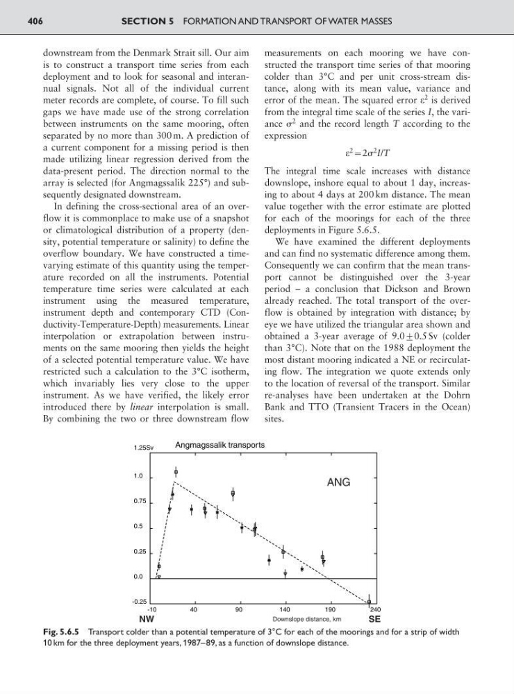
The integral time scale increases with distance
downslope, inshore equal to about 1 day, increasing to about 4 days at 200 km distance. The mean
value together with the error estimate are plotted
for each of the moorings for each of the three
deployments in Figure 5.6.5.
We have examined the different deployments
and can find no systematic difference among them.
Consequently we can confirm that the mean transport cannot be distinguished over the 3-year
period – a conclusion that Dickson and Brown
already reached. The total transport of the overflow is obtained by integration with distance; by
eye we have utilized the triangular area shown and
obtained a 3-year average of 9.0<0.5 Sv (colder
than 3°C). Note that on the 1988 deployment the
most distant mooring indicated a NE or recirculating flow. The integration we quote extends only
to the location of reversal of the transport. Similar
re-analyses have been undertaken at the Dohrn
Bank and TTO (Transient Tracers in the Ocean)
sites.
SECTION 5 FORMATION AND TRANSPORT OF WATER MASSES
406
Angmagssalik transports
-10
40
90
140
190
240
-0.25
0.0
0.25
0.5
0.75
1.0
1.25Sv
Downslope distance, km
SE
NW
ANG
Fig. 5.6.5 Transport colder than a potential temperature of 3°C for each of the moorings and for a strip of width
10 km for the three deployment years, 1987–89, as a function of downslope distance.
is to construct a transport time series from each
deployment and to look for seasonal and interannual signals. Not all of the individual current
meter records are complete, of course. To fill such
gaps we have made use of the strong correlation
between instruments on the same mooring, often
separated by no more than 300 m. A prediction of
a current component for a missing period is then
made utilizing linear regression derived from the
data-present period. The direction normal to the
array is selected (for Angmagssalik 225°) and subsequently designated downstream.
In defining the cross-sectional area of an overflow it is commonplace to make use of a snapshot
or climatological distribution of a property (density, potential temperature or salinity) to define the
overflow boundary. We have constructed a timevarying estimate of this quantity using the temperature recorded on all the instruments. Potential
temperature time series were calculated at each
instrument using the measured temperature,
instrument depth and contemporary CTD (Conductivity-Temperature-Depth) measurements. Linear
interpolation or extrapolation between instruments on the same mooring then yields the height
of a selected potential temperature value. We have
restricted such a calculation to the 3°C isotherm,
which invariably lies very close to the upper
instrument. As we have verified, the likely error
introduced there by linear interpolation is small.
By combining the two or three downstream flow
measurements on each mooring we have constructed the transport time series of that mooring
colder than 3°C and per unit cross-stream distance, along with its mean value, variance and
error of the mean. The squared error
2 is derived
from the integral time scale of the series I, the variance
2 and the record length T according to the
expression
2
:2
2 I/T
The integral time scale increases with distance
downslope, inshore equal to about 1 day, increasing to about 4 days at 200 km distance. The mean
value together with the error estimate are plotted
for each of the moorings for each of the three
deployments in Figure 5.6.5.
We have examined the different deployments
and can find no systematic difference among them.
Consequently we can confirm that the mean transport cannot be distinguished over the 3-year
period – a conclusion that Dickson and Brown
already reached. The total transport of the overflow is obtained by integration with distance; by
eye we have utilized the triangular area shown and
obtained a 3-year average of 9.0<0.5 Sv (colder
than 3°C). Note that on the 1988 deployment the
most distant mooring indicated a NE or recirculating flow. The integration we quote extends only
to the location of reversal of the transport. Similar
re-analyses have been undertaken at the Dohrn
Bank and TTO (Transient Tracers in the Ocean)
sites.
SECTION 5 FORMATION AND TRANSPORT OF WATER MASSES
406
Angmagssalik transports
-10
40
90
140
190
240
-0.25
0.0
0.25
0.5
0.75
1.0
1.25Sv
Downslope distance, km
SE
NW
ANG
Fig. 5.6.5 Transport colder than a potential temperature of 3°C for each of the moorings and for a strip of width
10 km for the three deployment years, 1987–89, as a function of downslope distance.