

rather rapid event marked by a rapid increase in
stratification, especially in the upper layers. One of
the best observations of restratification over a
larger area was obtained from a tomographic
array that integrates the water properties over the
array to give a larger-scale picture than a single
mooring can. This was obtained in the Golfe du
Lion by Send et al. (1995), who found a period of
restratification after the end of convection lasting
Ϸ40 days. Another example is the salinity record
from P-ALACE float 392 in the Labrador Sea
(Davis, 1998a; see also Davis and Zenk, Chapter
3.2). This shows, in early 1996 and 1997 in the
central Labrador Sea, a sudden transition between
the low stratification associated with convection
and a stratified water column. This record is
admittedly like a mooring, from a single point, but
it does give a consistent picture in the 2 years.
The restratification process has been modelled
numerically by Jones and Marshall (1997), who
envisage a homogeneous cylinder of water floating
in an ocean of constant stratification. The density
gradient between the cylinder and the surrounding
ocean gives rise to a narrow cyclonic current that
breaks up via baroclinic instability into baroclinic
eddies. These horizontally mix the homogeneous
water with the stratified waters, dissipating the
homogeneous cylinder in time scale, . For the special case where the stratification in the water
surrounding the homogeneous cylinder is concentrated in the upper layer, h,
Ϸ56r/(h⌬b)
1/2
where r is the radius of the homogeneous cylinder,
h is the depth of the upper stratified water bounding the homogeneous cylinder and ⌬b is the difference in density between the homogeneous water and
the surrounding water in buoyancy units. For the
Labrador Sea where hϷ500 m, ⌬bϷ210
93 m s
92
and rϷ100 km, Ϸ65 days. This result is about
twice the 1-month time scale for the rapid restratification but one-fifth of the 10-month time
scale for the slow restratification suggested in
Figure 5.5.5 (see Plate 5.5.5, p. 428). This suggests
the modelling result is more applicable to the rapid
phase of restratification.
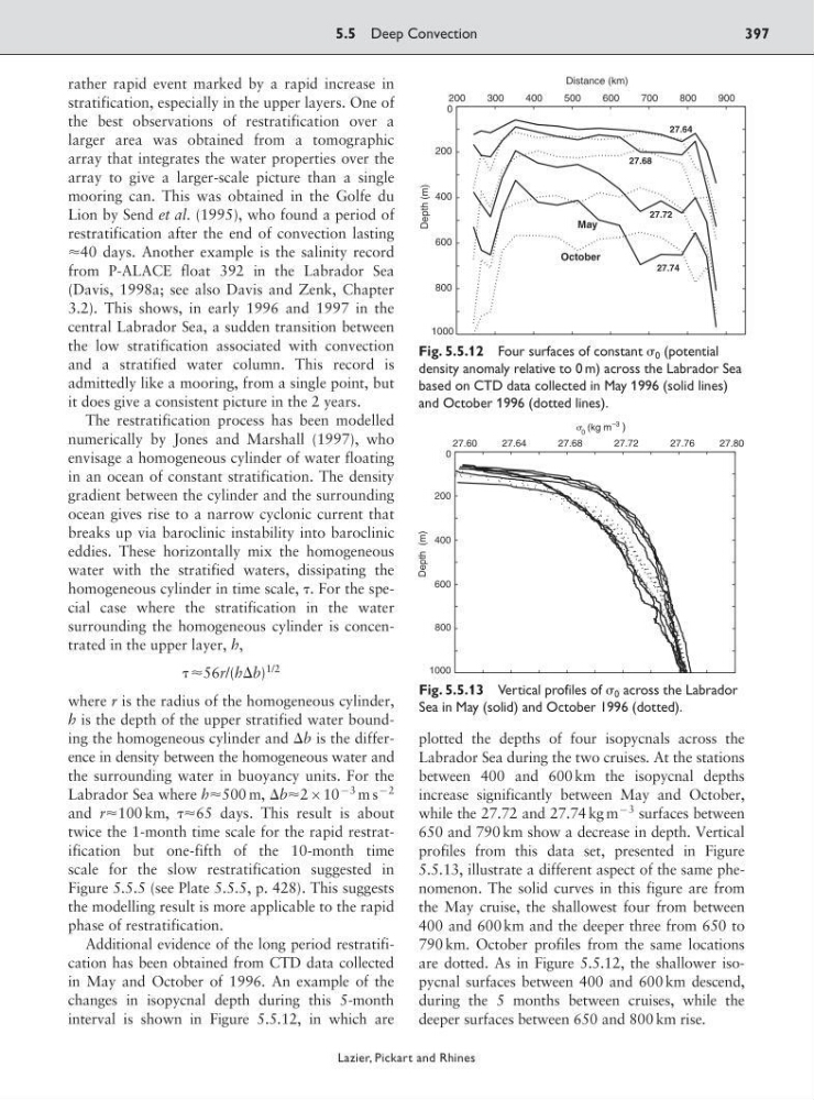
Additional evidence of the long period restratification has been obtained from CTD data collected
in May and October of 1996. An example of the
changes in isopycnal depth during this 5-month
interval is shown in Figure 5.5.12, in which are
plotted the depths of four isopycnals across the
Labrador Sea during the two cruises. At the stations
between 400 and 600 km the isopycnal depths
increase significantly between May and October,
while the 27.72 and 27.74 kg m
93 surfaces between
650 and 790 km show a decrease in depth. Vertical
profiles from this data set, presented in Figure
5.5.13, illustrate a different aspect of the same phenomenon. The solid curves in this figure are from
the May cruise, the shallowest four from between
400 and 600 km and the deeper three from 650 to
790 km. October profiles from the same locations
are dotted. As in Figure 5.5.12, the shallower isopycnal surfaces between 400 and 600 km descend,
during the 5 months between cruises, while the
deeper surfaces between 650 and 800 km rise.
5.5 Deep Convection
397
Lazier, Pickart and Rhines
200
300
400
500
600
700
800
900
1000
800
600
400
200
0
Distance (km)
Depth (m)
27.64
27.68
27.72
27.74
May
October
Fig. 5.5.12 Four surfaces of constant 0 (potential
density anomaly relative to 0 m) across the Labrador Sea
based on CTD data collected in May 1996 (solid lines)
and October 1996 (dotted lines).
27.60
27.64
27.68
27.72
27.76
27.80
1000
800
600
400
200
0
Depth (m)
(kg m )
0
–3
Fig. 5.5.13 Vertical profiles of 0 across the Labrador
Sea in May (solid) and October 1996 (dotted).
stratification, especially in the upper layers. One of
the best observations of restratification over a
larger area was obtained from a tomographic
array that integrates the water properties over the
array to give a larger-scale picture than a single
mooring can. This was obtained in the Golfe du
Lion by Send et al. (1995), who found a period of
restratification after the end of convection lasting
Ϸ40 days. Another example is the salinity record
from P-ALACE float 392 in the Labrador Sea
(Davis, 1998a; see also Davis and Zenk, Chapter
3.2). This shows, in early 1996 and 1997 in the
central Labrador Sea, a sudden transition between
the low stratification associated with convection
and a stratified water column. This record is
admittedly like a mooring, from a single point, but
it does give a consistent picture in the 2 years.
The restratification process has been modelled
numerically by Jones and Marshall (1997), who
envisage a homogeneous cylinder of water floating
in an ocean of constant stratification. The density
gradient between the cylinder and the surrounding
ocean gives rise to a narrow cyclonic current that
breaks up via baroclinic instability into baroclinic
eddies. These horizontally mix the homogeneous
water with the stratified waters, dissipating the
homogeneous cylinder in time scale, . For the special case where the stratification in the water
surrounding the homogeneous cylinder is concentrated in the upper layer, h,
Ϸ56r/(h⌬b)
1/2
where r is the radius of the homogeneous cylinder,
h is the depth of the upper stratified water bounding the homogeneous cylinder and ⌬b is the difference in density between the homogeneous water and
the surrounding water in buoyancy units. For the
Labrador Sea where hϷ500 m, ⌬bϷ210
93 m s
92
and rϷ100 km, Ϸ65 days. This result is about
twice the 1-month time scale for the rapid restratification but one-fifth of the 10-month time
scale for the slow restratification suggested in
Figure 5.5.5 (see Plate 5.5.5, p. 428). This suggests
the modelling result is more applicable to the rapid
phase of restratification.
Additional evidence of the long period restratification has been obtained from CTD data collected
in May and October of 1996. An example of the
changes in isopycnal depth during this 5-month
interval is shown in Figure 5.5.12, in which are
plotted the depths of four isopycnals across the
Labrador Sea during the two cruises. At the stations
between 400 and 600 km the isopycnal depths
increase significantly between May and October,
while the 27.72 and 27.74 kg m
93 surfaces between
650 and 790 km show a decrease in depth. Vertical
profiles from this data set, presented in Figure
5.5.13, illustrate a different aspect of the same phenomenon. The solid curves in this figure are from
the May cruise, the shallowest four from between
400 and 600 km and the deeper three from 650 to
790 km. October profiles from the same locations
are dotted. As in Figure 5.5.12, the shallower isopycnal surfaces between 400 and 600 km descend,
during the 5 months between cruises, while the
deeper surfaces between 650 and 800 km rise.
5.5 Deep Convection
397
Lazier, Pickart and Rhines
200
300
400
500
600
700
800
900
1000
800
600
400
200
0
Distance (km)
Depth (m)
27.64
27.68
27.72
27.74
May
October
Fig. 5.5.12 Four surfaces of constant 0 (potential
density anomaly relative to 0 m) across the Labrador Sea
based on CTD data collected in May 1996 (solid lines)
and October 1996 (dotted lines).
27.60
27.64
27.68
27.72
27.76
27.80
1000
800
600
400
200
0
Depth (m)
(kg m )
0
–3
Fig. 5.5.13 Vertical profiles of 0 across the Labrador
Sea in May (solid) and October 1996 (dotted).