

This feature is typical of atmospheric numerical
models, is due to an erroneous ITCZ south of the
equator, and is one major difficulty in using such
analyses. This artefact is also evident in the ensemble average of Wijffels (Chapter 6.2), which also
shows more net freshwater flux in the western tropical Pacific and eastern tropical Indian Ocean. Otherwise, the two fields are not significantly different.
There is nothing unexpected in the zonal average freshwater flux (not shown) from Figure
5.1.11. There are maxima at 52°N, 6°N and
between 45 and 60°S at 20, 37 and 15 mg m
92 s
91
,
respectively. The minima at 20°S and 22°N are
both about 926 mg m
92 s
91
. The northward
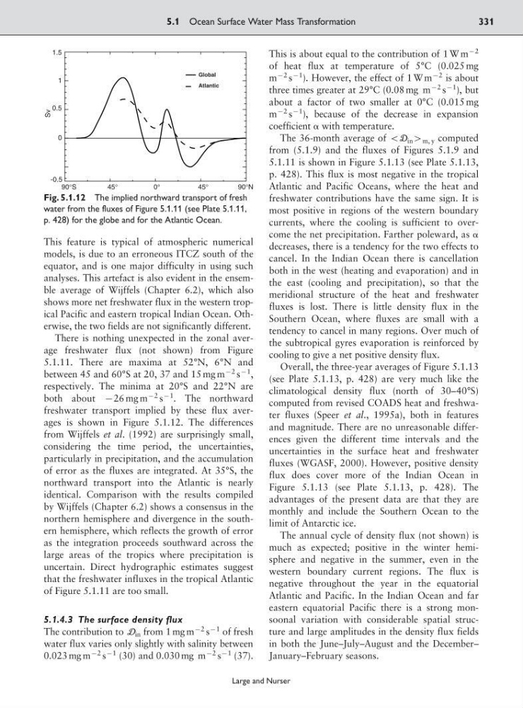
freshwater transport implied by these flux averages is shown in Figure 5.1.12. The differences
from Wijffels et al. (1992) are surprisingly small,
considering the time period, the uncertainties,
particularly in precipitation, and the accumulation
of error as the fluxes are integrated. At 35°S, the
northward transport into the Atlantic is nearly
identical. Comparison with the results compiled
by Wijffels (Chapter 6.2) shows a consensus in the
northern hemisphere and divergence in the southern hemisphere, which reflects the growth of error
as the integration proceeds southward across the
large areas of the tropics where precipitation is
uncertain. Direct hydrographic estimates suggest
that the freshwater influxes in the tropical Atlantic
of Figure 5.1.11 are too small.
5.1.4.3 The surface density flux
The contribution to D in from 1 mg m
92 s
91 of fresh
water flux varies only slightly with salinity between
0.023 mg m
92 s
91 (30) and 0.030 mg m
92 s
91 (37).
This is about equal to the contribution of 1 W m
92
of heat flux at temperature of 5°C (0.025 mg
m
92 s
91
). However, the effect of 1 W m
92 is about
three times greater at 29°C (0.08 mg m
92 s
91
), but
about a factor of two smaller at 0°C (0.015 mg
m
92 s
91
), because of the decrease in expansion
coefficient ␣ with temperature.
The 36-month average of :D in 9 m, y computed
from (5.1.9) and the fluxes of Figures 5.1.9 and
5.1.11 is shown in Figure 5.1.13 (see Plate 5.1.13,
p. 428). This flux is most negative in the tropical
Atlantic and Pacific Oceans, where the heat and
freshwater contributions have the same sign. It is
most positive in regions of the western boundary
currents, where the cooling is sufficient to overcome the net precipitation. Farther poleward, as ␣
decreases, there is a tendency for the two effects to
cancel. In the Indian Ocean there is cancellation
both in the west (heating and evaporation) and in
the east (cooling and precipitation), so that the
meridional structure of the heat and freshwater
fluxes is lost. There is little density flux in the
Southern Ocean, where fluxes are small with a
tendency to cancel in many regions. Over much of
the subtropical gyres evaporation is reinforced by
cooling to give a net positive density flux.
Overall, the three-year averages of Figure 5.1.13
(see Plate 5.1.13, p. 428) are very much like the
climatological density flux (north of 30–40°S)
computed from revised COADS heat and freshwater fluxes (Speer et al., 1995a), both in features
and magnitude. There are no unreasonable differences given the different time intervals and the
uncertainties in the surface heat and freshwater
fluxes (WGASF, 2000). However, positive density
flux does cover more of the Indian Ocean in
Figure 5.1.13 (see Plate 5.1.13, p. 428). The
advantages of the present data are that they are
monthly and include the Southern Ocean to the
limit of Antarctic ice.
The annual cycle of density flux (not shown) is
much as expected; positive in the winter hemisphere and negative in the summer, even in the
western boundary current regions. The flux is
negative throughout the year in the equatorial
Atlantic and Pacific. In the Indian Ocean and far
eastern equatorial Pacific there is a strong monsoonal variation with considerable spatial structure and large amplitudes in the density flux fields
in both the June–July–August and the December–
January–February seasons.
5.1 Ocean Surface Water Mass Transformation
331
Large and Nurser
1.5
1
0.5
0
-0.5
Sv
90°S
4 5 °
45°
0°
90°N
Global
Atlantic
Fig. 5.1.12 The implied northward transport of fresh
water from the fluxes of Figure 5.1.11 (see Plate 5.1.11,
p. 428) for the globe and for the Atlantic Ocean.
models, is due to an erroneous ITCZ south of the
equator, and is one major difficulty in using such
analyses. This artefact is also evident in the ensemble average of Wijffels (Chapter 6.2), which also
shows more net freshwater flux in the western tropical Pacific and eastern tropical Indian Ocean. Otherwise, the two fields are not significantly different.
There is nothing unexpected in the zonal average freshwater flux (not shown) from Figure
5.1.11. There are maxima at 52°N, 6°N and
between 45 and 60°S at 20, 37 and 15 mg m
92 s
91
,
respectively. The minima at 20°S and 22°N are
both about 926 mg m
92 s
91
. The northward
freshwater transport implied by these flux averages is shown in Figure 5.1.12. The differences
from Wijffels et al. (1992) are surprisingly small,
considering the time period, the uncertainties,
particularly in precipitation, and the accumulation
of error as the fluxes are integrated. At 35°S, the
northward transport into the Atlantic is nearly
identical. Comparison with the results compiled
by Wijffels (Chapter 6.2) shows a consensus in the
northern hemisphere and divergence in the southern hemisphere, which reflects the growth of error
as the integration proceeds southward across the
large areas of the tropics where precipitation is
uncertain. Direct hydrographic estimates suggest
that the freshwater influxes in the tropical Atlantic
of Figure 5.1.11 are too small.
5.1.4.3 The surface density flux
The contribution to D in from 1 mg m
92 s
91 of fresh
water flux varies only slightly with salinity between
0.023 mg m
92 s
91 (30) and 0.030 mg m
92 s
91 (37).
This is about equal to the contribution of 1 W m
92
of heat flux at temperature of 5°C (0.025 mg
m
92 s
91
). However, the effect of 1 W m
92 is about
three times greater at 29°C (0.08 mg m
92 s
91
), but
about a factor of two smaller at 0°C (0.015 mg
m
92 s
91
), because of the decrease in expansion
coefficient ␣ with temperature.
The 36-month average of :D in 9 m, y computed
from (5.1.9) and the fluxes of Figures 5.1.9 and
5.1.11 is shown in Figure 5.1.13 (see Plate 5.1.13,
p. 428). This flux is most negative in the tropical
Atlantic and Pacific Oceans, where the heat and
freshwater contributions have the same sign. It is
most positive in regions of the western boundary
currents, where the cooling is sufficient to overcome the net precipitation. Farther poleward, as ␣
decreases, there is a tendency for the two effects to
cancel. In the Indian Ocean there is cancellation
both in the west (heating and evaporation) and in
the east (cooling and precipitation), so that the
meridional structure of the heat and freshwater
fluxes is lost. There is little density flux in the
Southern Ocean, where fluxes are small with a
tendency to cancel in many regions. Over much of
the subtropical gyres evaporation is reinforced by
cooling to give a net positive density flux.
Overall, the three-year averages of Figure 5.1.13
(see Plate 5.1.13, p. 428) are very much like the
climatological density flux (north of 30–40°S)
computed from revised COADS heat and freshwater fluxes (Speer et al., 1995a), both in features
and magnitude. There are no unreasonable differences given the different time intervals and the
uncertainties in the surface heat and freshwater
fluxes (WGASF, 2000). However, positive density
flux does cover more of the Indian Ocean in
Figure 5.1.13 (see Plate 5.1.13, p. 428). The
advantages of the present data are that they are
monthly and include the Southern Ocean to the
limit of Antarctic ice.
The annual cycle of density flux (not shown) is
much as expected; positive in the winter hemisphere and negative in the summer, even in the
western boundary current regions. The flux is
negative throughout the year in the equatorial
Atlantic and Pacific. In the Indian Ocean and far
eastern equatorial Pacific there is a strong monsoonal variation with considerable spatial structure and large amplitudes in the density flux fields
in both the June–July–August and the December–
January–February seasons.
5.1 Ocean Surface Water Mass Transformation
331
Large and Nurser
1.5
1
0.5
0
-0.5
Sv
90°S
4 5 °
45°
0°
90°N
Global
Atlantic
Fig. 5.1.12 The implied northward transport of fresh
water from the fluxes of Figure 5.1.11 (see Plate 5.1.11,
p. 428) for the globe and for the Atlantic Ocean.