

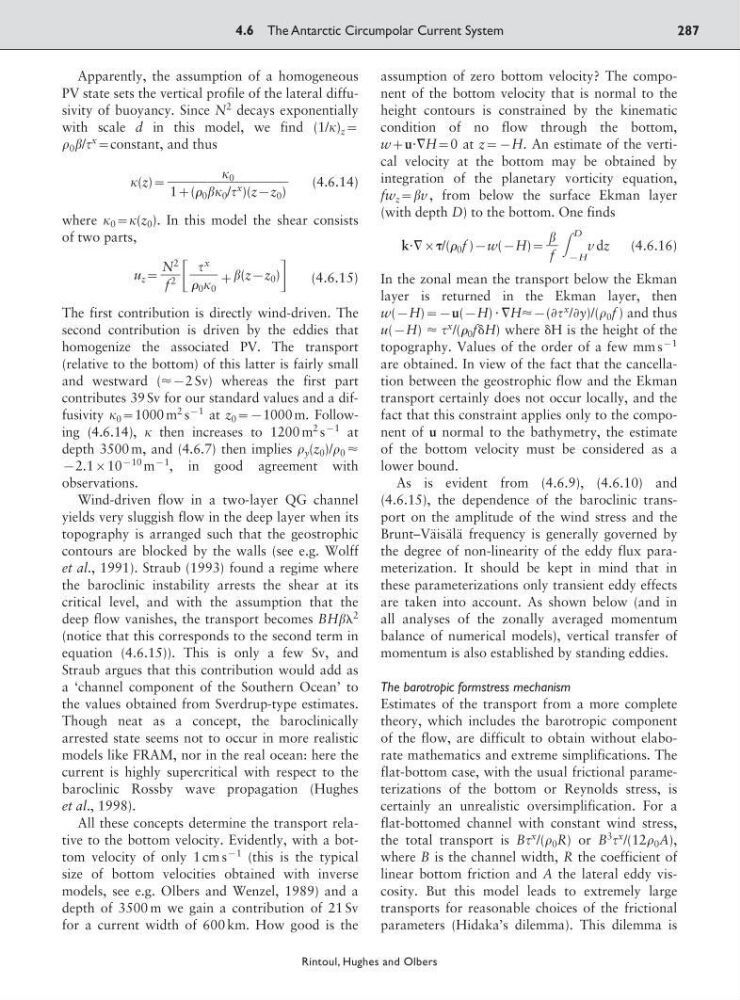
Apparently, the assumption of a homogeneous
PV state sets the vertical profile of the lateral diffusivity of buoyancy. Since N
2 decays exponentially
with scale d in this model, we find (1/) z :
0 /
x
:constant, and thus
(z):
(4.6.14)
where 0 :(z 0 ). In this model the shear consists
of two parts,
u z :
΄ ; (z9z 0 ) ΅ (4.6.15)
The first contribution is directly wind-driven. The
second contribution is driven by the eddies that
homogenize the associated PV. The transport
(relative to the bottom) of this latter is fairly small
and westward (Ϸ92 Sv) whereas the first part
contributes 39 Sv for our standard values and a diffusivity 0 :1000 m
2 s
91 at z 0 :91000 m. Following (4.6.14), then increases to 1200 m
2 s
91 at
depth 3500 m, and (4.6.7) then implies y (z 0 )/ 0 Ϸ
92.110
910 m
91
, in good agreement with
observations.
Wind-driven flow in a two-layer QG channel
yields very sluggish flow in the deep layer when its
topography is arranged such that the geostrophic
contours are blocked by the walls (see e.g. Wolff
et al., 1991). Straub (1993) found a regime where
the baroclinic instability arrests the shear at its
critical level, and with the assumption that the
deep flow vanishes, the transport becomes BH
2
(notice that this corresponds to the second term in
equation (4.6.15)). This is only a few Sv, and
Straub argues that this contribution would add as
a ‘channel component of the Southern Ocean’ to
the values obtained from Sverdrup-type estimates.
Though neat as a concept, the baroclinically
arrested state seems not to occur in more realistic
models like FRAM, nor in the real ocean: here the
current is highly supercritical with respect to the
baroclinic Rossby wave propagation (Hughes
et al., 1998).
All these concepts determine the transport relative to the bottom velocity. Evidently, with a bottom velocity of only 1 cm s
91 (this is the typical
size of bottom velocities obtained with inverse
models, see e.g. Olbers and Wenzel, 1989) and a
depth of 3500 m we gain a contribution of 21 Sv
for a current width of 600 km. How good is the
assumption of zero bottom velocity? The component of the bottom velocity that is normal to the
height contours is constrained by the kinematic
condition of no flow through the bottom,
w;uиٌH:0 at z:9H. An estimate of the vertical velocity at the bottom may be obtained by
integration of the planetary vorticity equation,
fw z :v , from below the surface Ekman layer
(with depth D) to the bottom. One finds
kиٌ/( 0 f )9w(9H): ͵
D
9H
v dz
(4.6.16)
In the zonal mean the transport below the Ekman
layer is returned in the Ekman layer, then
w(9H):9u(9H) и ٌHϷ9(Ѩ
x
/Ѩy)/( 0 f ) and thus
u(9H) Ϸ
x
/( 0 f␦H) where ␦H is the height of the
topography. Values of the order of a few mm s
91
are obtained. In view of the fact that the cancellation between the geostrophic flow and the Ekman
transport certainly does not occur locally, and the
fact that this constraint applies only to the component of u normal to the bathymetry, the estimate
of the bottom velocity must be considered as a
lower bound.
As is evident from (4.6.9), (4.6.10) and
(4.6.15), the dependence of the baroclinic transport on the amplitude of the wind stress and the
Brunt–Väisälä frequency is generally governed by
the degree of non-linearity of the eddy flux parameterization. It should be kept in mind that in
these parameterizations only transient eddy effects
are taken into account. As shown below (and in
all analyses of the zonally averaged momentum
balance of numerical models), vertical transfer of
momentum is also established by standing eddies.
The barotropic formstress mechanism
Estimates of the transport from a more complete
theory, which includes the barotropic component
of the flow, are difficult to obtain without elaborate mathematics and extreme simplifications. The
flat-bottom case, with the usual frictional parameterizations of the bottom or Reynolds stress, is
certainly an unrealistic oversimplification. For a
flat-bottomed channel with constant wind stress,
the total transport is B
x
/( 0 R) or B
3
x
/(12 0 A),
where B is the channel width, R the coefficient of
linear bottom friction and A the lateral eddy viscosity. But this model leads to extremely large
transports for reasonable choices of the frictional
parameters (Hidaka’s dilemma). This dilemma is
ᎏ
f
x
ᎏ
0 0
N
2
ᎏ
f
2
0
ᎏᎏᎏ
1;( 0 0 /
x
)(z9z 0 )
4.6 The Antarctic Circumpolar Current System
287
Rintoul, Hughes and Olbers
PV state sets the vertical profile of the lateral diffusivity of buoyancy. Since N
2 decays exponentially
with scale d in this model, we find (1/) z :
0 /
x
:constant, and thus
(z):
(4.6.14)
where 0 :(z 0 ). In this model the shear consists
of two parts,
u z :
΄ ; (z9z 0 ) ΅ (4.6.15)
The first contribution is directly wind-driven. The
second contribution is driven by the eddies that
homogenize the associated PV. The transport
(relative to the bottom) of this latter is fairly small
and westward (Ϸ92 Sv) whereas the first part
contributes 39 Sv for our standard values and a diffusivity 0 :1000 m
2 s
91 at z 0 :91000 m. Following (4.6.14), then increases to 1200 m
2 s
91 at
depth 3500 m, and (4.6.7) then implies y (z 0 )/ 0 Ϸ
92.110
910 m
91
, in good agreement with
observations.
Wind-driven flow in a two-layer QG channel
yields very sluggish flow in the deep layer when its
topography is arranged such that the geostrophic
contours are blocked by the walls (see e.g. Wolff
et al., 1991). Straub (1993) found a regime where
the baroclinic instability arrests the shear at its
critical level, and with the assumption that the
deep flow vanishes, the transport becomes BH
2
(notice that this corresponds to the second term in
equation (4.6.15)). This is only a few Sv, and
Straub argues that this contribution would add as
a ‘channel component of the Southern Ocean’ to
the values obtained from Sverdrup-type estimates.
Though neat as a concept, the baroclinically
arrested state seems not to occur in more realistic
models like FRAM, nor in the real ocean: here the
current is highly supercritical with respect to the
baroclinic Rossby wave propagation (Hughes
et al., 1998).
All these concepts determine the transport relative to the bottom velocity. Evidently, with a bottom velocity of only 1 cm s
91 (this is the typical
size of bottom velocities obtained with inverse
models, see e.g. Olbers and Wenzel, 1989) and a
depth of 3500 m we gain a contribution of 21 Sv
for a current width of 600 km. How good is the
assumption of zero bottom velocity? The component of the bottom velocity that is normal to the
height contours is constrained by the kinematic
condition of no flow through the bottom,
w;uиٌH:0 at z:9H. An estimate of the vertical velocity at the bottom may be obtained by
integration of the planetary vorticity equation,
fw z :v , from below the surface Ekman layer
(with depth D) to the bottom. One finds
kиٌ/( 0 f )9w(9H): ͵
D
9H
v dz
(4.6.16)
In the zonal mean the transport below the Ekman
layer is returned in the Ekman layer, then
w(9H):9u(9H) и ٌHϷ9(Ѩ
x
/Ѩy)/( 0 f ) and thus
u(9H) Ϸ
x
/( 0 f␦H) where ␦H is the height of the
topography. Values of the order of a few mm s
91
are obtained. In view of the fact that the cancellation between the geostrophic flow and the Ekman
transport certainly does not occur locally, and the
fact that this constraint applies only to the component of u normal to the bathymetry, the estimate
of the bottom velocity must be considered as a
lower bound.
As is evident from (4.6.9), (4.6.10) and
(4.6.15), the dependence of the baroclinic transport on the amplitude of the wind stress and the
Brunt–Väisälä frequency is generally governed by
the degree of non-linearity of the eddy flux parameterization. It should be kept in mind that in
these parameterizations only transient eddy effects
are taken into account. As shown below (and in
all analyses of the zonally averaged momentum
balance of numerical models), vertical transfer of
momentum is also established by standing eddies.
The barotropic formstress mechanism
Estimates of the transport from a more complete
theory, which includes the barotropic component
of the flow, are difficult to obtain without elaborate mathematics and extreme simplifications. The
flat-bottom case, with the usual frictional parameterizations of the bottom or Reynolds stress, is
certainly an unrealistic oversimplification. For a
flat-bottomed channel with constant wind stress,
the total transport is B
x
/( 0 R) or B
3
x
/(12 0 A),
where B is the channel width, R the coefficient of
linear bottom friction and A the lateral eddy viscosity. But this model leads to extremely large
transports for reasonable choices of the frictional
parameters (Hidaka’s dilemma). This dilemma is
ᎏ
f
x
ᎏ
0 0
N
2
ᎏ
f
2
0
ᎏᎏᎏ
1;( 0 0 /
x
)(z9z 0 )
4.6 The Antarctic Circumpolar Current System
287
Rintoul, Hughes and Olbers