

When the altimetric estimates of heat storage
change are averaged over large ocean basins, the
errors caused by non-thermally related sea-level
signals tend to be averaged out, leading to a fairly
accurate estimate of basin-wide heat flux change.
However, such error reduction does not apply to
regional analysis. For instance, the effects of heat
advection by ocean currents become important in
the regions of the Kuroshio Extension and the
Gulf Stream. In an effort to investigate the utility
of altimetry data for diagnosing the heat budget of
the ocean, Qiu and Kelly (1993) used a numerical
model of the ocean’s mixed layer driven by wind
and heat flux with the geostrophic current velocity
estimated from GEOSAT observations for estimating the mixed-layer depth and temperature of the
Kuroshio Extension region. They found that the
advection of heat by the surface flows made a substantial contribution to the local heat balance. The
advection warms the upstream region of the
Kuroshio Extension while it cools the downstream
region due to the presence of the recirculation
gyre. Using a similar approach, Kelly and Qiu
(1995a,b) ran the mixed-layer model with assimilation of altimeter data and sea surface temperature data for studying the heat balance of the Gulf
Stream gyre. Rather than forcing the model with
heat flux produced by weather centres, heat flux
was estimated as the residual of the heat budget
that involved horizontal advection, vertical
entrainment, and eddy diffusion. The error in the
heat flux estimate ranges from 20 to 100 W m
92
.
Based on the heat budget analysis, the seasonal
variability of the heat content of the gyre to the
south of the Gulf Stream is primarily forced by the
air–sea heat flux (also see Wang and Koblinsky,
1996). Within the Gulf Stream and to the north of
it, the cooling by the southward Ekman advection
of cold water has a tendency to be balanced by
the warming of the Gulf Stream. A very complex
pattern of air–sea interaction was present in the
region, showing coupling between the air–sea heat
flux and the wind-driven circulation (also see Kelly
et al., 1999).
Wind-forced variability
Wind stress exerts forcing on the ocean over a wide
range of spatial and temporal scales. The ocean’s
response is complicated, involving both local
adjustment and propagating waves from remote
forcing. The vertical structure of the ocean’s
response is a function of the spatial and temporal
scales of the forcing. The relation between windforced sea-level variability and the internal structure
of the oceanic variability is thus scale-dependent.
Outside the tropics, the ocean’s response to
time-varying wind forcing at large scales is primarily through the vertical motion caused by the
convergence/divergence of the Ekman flow in the
surface layer driven by the curl of wind stress, the
Ekman pumping (e.g. Pedlosky, 1987b). Depending on the spatial and temporal scales of the
forcing, the ocean’s response has different vertical
structures. At spatial scales larger than 1000 km
and time scales shorter than 300 days, the ocean’s
response is primarily barotropic, or depth independent (Willebrand et al., 1980; Koblinsky et al.,
1989; Fukumori et al., 1998). Sea level is then a
good indicator of the motion of the entire water
column and can be described to a large extent by
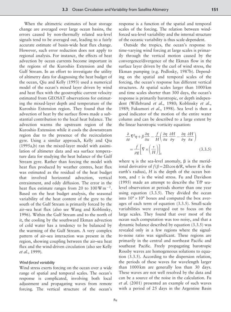
the linear barotropic vorticity equation:
ٌ
2
;
9
9
:
΄ ٌ ΅ z
(3.3.5)
where is the sea-level anomaly,  is the meridional derivative of f (:2⍀ cos /R, where R is the
earth’s radius), H is the depth of the ocean bottom, and is the wind stress. Fu and Davidson
(1995) made an attempt to describe the T/P sealevel observation at periods shorter than one year
using equation (3.3.5). They divided the ocean
into 10°10° boxes and computed the box averages of each term of equation (3.3.5). Small-scale
variabilities were averaged out to focus on the
large scales. They found that over most of the
ocean such computation was too noisy, and that a
dynamic balance described by equation (3.3.5) was
revealed only in a few regions where the signalto-noise ratio was significant. These regions are
primarily in the central and northeast Pacific and
southeast Pacific. Freely propagating barotropic
Rossby waves are homogeneous solutions to equation (3.3.5). According to the dispersion relation,
the periods of these waves for wavelength larger
than 1000 km are generally less than 30 days.
These waves are not well resolved by the data and
can be a source of the noise in the calculation. Fu
et al. (2001) presented an example of such waves
with a period of 25 days in the Argentine Basin
ᎏ
H
f
ᎏ
g
ѨH
ᎏ
Ѩx
Ѩ
ᎏ
Ѩy
ѨH
ᎏ
Ѩy
Ѩ
ᎏ
Ѩx
f
ᎏ
H
Ѩ
ᎏ
Ѩx
Ѩ
ᎏ
Ѩt
3.3 Ocean Circulation and Variability from Satellite Altimetry
151
Fu
change are averaged over large ocean basins, the
errors caused by non-thermally related sea-level
signals tend to be averaged out, leading to a fairly
accurate estimate of basin-wide heat flux change.
However, such error reduction does not apply to
regional analysis. For instance, the effects of heat
advection by ocean currents become important in
the regions of the Kuroshio Extension and the
Gulf Stream. In an effort to investigate the utility
of altimetry data for diagnosing the heat budget of
the ocean, Qiu and Kelly (1993) used a numerical
model of the ocean’s mixed layer driven by wind
and heat flux with the geostrophic current velocity
estimated from GEOSAT observations for estimating the mixed-layer depth and temperature of the
Kuroshio Extension region. They found that the
advection of heat by the surface flows made a substantial contribution to the local heat balance. The
advection warms the upstream region of the
Kuroshio Extension while it cools the downstream
region due to the presence of the recirculation
gyre. Using a similar approach, Kelly and Qiu
(1995a,b) ran the mixed-layer model with assimilation of altimeter data and sea surface temperature data for studying the heat balance of the Gulf
Stream gyre. Rather than forcing the model with
heat flux produced by weather centres, heat flux
was estimated as the residual of the heat budget
that involved horizontal advection, vertical
entrainment, and eddy diffusion. The error in the
heat flux estimate ranges from 20 to 100 W m
92
.
Based on the heat budget analysis, the seasonal
variability of the heat content of the gyre to the
south of the Gulf Stream is primarily forced by the
air–sea heat flux (also see Wang and Koblinsky,
1996). Within the Gulf Stream and to the north of
it, the cooling by the southward Ekman advection
of cold water has a tendency to be balanced by
the warming of the Gulf Stream. A very complex
pattern of air–sea interaction was present in the
region, showing coupling between the air–sea heat
flux and the wind-driven circulation (also see Kelly
et al., 1999).
Wind-forced variability
Wind stress exerts forcing on the ocean over a wide
range of spatial and temporal scales. The ocean’s
response is complicated, involving both local
adjustment and propagating waves from remote
forcing. The vertical structure of the ocean’s
response is a function of the spatial and temporal
scales of the forcing. The relation between windforced sea-level variability and the internal structure
of the oceanic variability is thus scale-dependent.
Outside the tropics, the ocean’s response to
time-varying wind forcing at large scales is primarily through the vertical motion caused by the
convergence/divergence of the Ekman flow in the
surface layer driven by the curl of wind stress, the
Ekman pumping (e.g. Pedlosky, 1987b). Depending on the spatial and temporal scales of the
forcing, the ocean’s response has different vertical
structures. At spatial scales larger than 1000 km
and time scales shorter than 300 days, the ocean’s
response is primarily barotropic, or depth independent (Willebrand et al., 1980; Koblinsky et al.,
1989; Fukumori et al., 1998). Sea level is then a
good indicator of the motion of the entire water
column and can be described to a large extent by
the linear barotropic vorticity equation:
ٌ
2
;
9
9
:
΄ ٌ ΅ z
(3.3.5)
where is the sea-level anomaly,  is the meridional derivative of f (:2⍀ cos /R, where R is the
earth’s radius), H is the depth of the ocean bottom, and is the wind stress. Fu and Davidson
(1995) made an attempt to describe the T/P sealevel observation at periods shorter than one year
using equation (3.3.5). They divided the ocean
into 10°10° boxes and computed the box averages of each term of equation (3.3.5). Small-scale
variabilities were averaged out to focus on the
large scales. They found that over most of the
ocean such computation was too noisy, and that a
dynamic balance described by equation (3.3.5) was
revealed only in a few regions where the signalto-noise ratio was significant. These regions are
primarily in the central and northeast Pacific and
southeast Pacific. Freely propagating barotropic
Rossby waves are homogeneous solutions to equation (3.3.5). According to the dispersion relation,
the periods of these waves for wavelength larger
than 1000 km are generally less than 30 days.
These waves are not well resolved by the data and
can be a source of the noise in the calculation. Fu
et al. (2001) presented an example of such waves
with a period of 25 days in the Argentine Basin
ᎏ
H
f
ᎏ
g
ѨH
ᎏ
Ѩx
Ѩ
ᎏ
Ѩy
ѨH
ᎏ
Ѩy
Ѩ
ᎏ
Ѩx
f
ᎏ
H
Ѩ
ᎏ
Ѩx
Ѩ
ᎏ
Ѩt
3.3 Ocean Circulation and Variability from Satellite Altimetry
151
Fu