

salinity effects on sea level are important in certain
regions (Maes, 1998; Sato et al., 2000). On global
scales, the contribution of freshwater exchange
between the ocean and the atmosphere is discernible in the seasonal variations of the global
mean sea level after the thermal effects are
removed (Minster et al., 1999).
Steric sea-level variability occurs over the scales
of air–sea heat and freshwater exchange, typically
on the order of 1000 km and larger. To study the
mechanisms of sea-level variability at these scales,
it is essential to be able to separate the steric
effects from others. To the extent that the steric
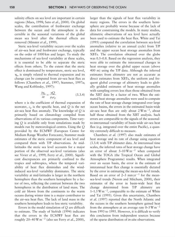
effect is dominated by temperature, steric sea level,
s , is simply related to thermal expansion and its
change can be computed from air–sea heat flux as
follows (Chambers et al., 1997; Stammer, 1997a;
Wang and Koblinsky, 1997):
:
(3.3.4)
where is the coefficient of thermal expansion of
seawater, c p is the specific heat, and Q is the net
air–sea heat flux anomaly. The knowledge of Q is
primarily based on climatology compiled from
observations of its various components. Time-varying Q is available only from simulations made by
models run by meteorological centres. Using the Q
provided by the ECMWF (European Centre for
Medium Range Weather Forecasts), Stammer made
estimates of the steric component of sea level and
compared them with T/P observations. At midlatitudes the steric sea level accounts for a major
portion of the observed sea-level variations (also
see Vivier et al., 1999; Ferry et al., 2000). Significant discrepancies are primarily confined to the
tropics and subtropics, where the temporal variability of heat flux diminishes and the windinduced sea-level variability dominates. The steric
variability at mid-latitudes is larger in the northern
hemisphere than the southern hemisphere by a factor of two, reflecting the contrast between the two
hemispheres in the distribution of land mass. The
cold air blown from the continents to the warm
oceans during winter time is a major contributor to
the air–sea heat flux. The lack of land mass in the
southern hemisphere leads to less steric variability.
Errors in the model simulation of Q are difficult
to estimate. The study of Siefridt (1994) indicates
that the errors in the ECMWF heat flux are
roughly 20–40 W m
92 (also see Ferry et al., 2000),
larger than the signals of heat flux variability in
many regions. The errors in the southern hemisphere are probably worse because of the lack of
data for constraining the models. In many studies,
altimetric observations of sea level have actually
been used to estimate the heat flux. White and Tai
(1995) computed the correlation between sea-level
anomalies (relative to an annual cycle) from T/P
and the upper ocean heat storage anomalies from
XBTs. The correlation obtained over the globe
was 0.5–0.8. Based on the regression analysis, they
were able to estimate the interannual changes in
heat storage over the global upper ocean (above
400 m) using the T/P data. Although the inferred
estimates from altimetry are not as accurate as
direct estimates from XBTs, the uniform and frequent global coverage of altimetry leads to globally gridded estimates of heat storage anomalies
with sampling errors less than those obtained from
the XBT data by a factor of two. When the estimated heat storage anomalies were used to compute
the rate of heat storage change integrated over large
ocean basins, the errors in the estimated basin-wide
air–sea heat flux are only about 2 W m
92
, about
half those obtained from the XBT analysis. Such
errors are comparable to the signals of the seasonalto-interannual variability of basin-wide air–sea heat
flux (e.g. integrated over the entire Pacific), a quantity extremely difficult to measure.
Chambers et al. (1997) also made estimates of
heat storage and its rate of change using equation
(3.3.4) with T/P altimeter data. At interannual time
scales, the inferred rates of heat storage change have
an error of about 5–10 W m
92 when compared
with the TOGA (the Tropical Ocean and Global
Atmosphere Programme) results. When integrated
over an ocean basin, the error in the estimate of
interannual heat flux change is essentially dictated
by the error in estimating the mean-sea-level trends.
Based on an error of 2–3 mm yr
91 for the meansea-level trends (Nerem and Mitchum, 2000), their
estimates of the error in basin-wide heat flux
change determined from T/P altimetry are
1–1.5 W m
92
, comparable to the estimate of White
and Tai (1995). Given this uncertainty, Chambers
et al. (1997) reported that the North Atlantic and
the oceans in the southern hemisphere gained heat
from the atmosphere at an average rate 0–3 W m
92
from 1993 to 1995. However, it is difficult to verify
this conclusion from independent sources because
of the sparse distribution of in-situ observations.
Q
ᎏ
0 c p
Ѩ s
ᎏ
Ѩt
SECTION 3 NEW WAYS OF OBSERVING THE OCEAN
150
regions (Maes, 1998; Sato et al., 2000). On global
scales, the contribution of freshwater exchange
between the ocean and the atmosphere is discernible in the seasonal variations of the global
mean sea level after the thermal effects are
removed (Minster et al., 1999).
Steric sea-level variability occurs over the scales
of air–sea heat and freshwater exchange, typically
on the order of 1000 km and larger. To study the
mechanisms of sea-level variability at these scales,
it is essential to be able to separate the steric
effects from others. To the extent that the steric
effect is dominated by temperature, steric sea level,
s , is simply related to thermal expansion and its
change can be computed from air–sea heat flux as
follows (Chambers et al., 1997; Stammer, 1997a;
Wang and Koblinsky, 1997):
:
(3.3.4)
where is the coefficient of thermal expansion of
seawater, c p is the specific heat, and Q is the net
air–sea heat flux anomaly. The knowledge of Q is
primarily based on climatology compiled from
observations of its various components. Time-varying Q is available only from simulations made by
models run by meteorological centres. Using the Q
provided by the ECMWF (European Centre for
Medium Range Weather Forecasts), Stammer made
estimates of the steric component of sea level and
compared them with T/P observations. At midlatitudes the steric sea level accounts for a major
portion of the observed sea-level variations (also
see Vivier et al., 1999; Ferry et al., 2000). Significant discrepancies are primarily confined to the
tropics and subtropics, where the temporal variability of heat flux diminishes and the windinduced sea-level variability dominates. The steric
variability at mid-latitudes is larger in the northern
hemisphere than the southern hemisphere by a factor of two, reflecting the contrast between the two
hemispheres in the distribution of land mass. The
cold air blown from the continents to the warm
oceans during winter time is a major contributor to
the air–sea heat flux. The lack of land mass in the
southern hemisphere leads to less steric variability.
Errors in the model simulation of Q are difficult
to estimate. The study of Siefridt (1994) indicates
that the errors in the ECMWF heat flux are
roughly 20–40 W m
92 (also see Ferry et al., 2000),
larger than the signals of heat flux variability in
many regions. The errors in the southern hemisphere are probably worse because of the lack of
data for constraining the models. In many studies,
altimetric observations of sea level have actually
been used to estimate the heat flux. White and Tai
(1995) computed the correlation between sea-level
anomalies (relative to an annual cycle) from T/P
and the upper ocean heat storage anomalies from
XBTs. The correlation obtained over the globe
was 0.5–0.8. Based on the regression analysis, they
were able to estimate the interannual changes in
heat storage over the global upper ocean (above
400 m) using the T/P data. Although the inferred
estimates from altimetry are not as accurate as
direct estimates from XBTs, the uniform and frequent global coverage of altimetry leads to globally gridded estimates of heat storage anomalies
with sampling errors less than those obtained from
the XBT data by a factor of two. When the estimated heat storage anomalies were used to compute
the rate of heat storage change integrated over large
ocean basins, the errors in the estimated basin-wide
air–sea heat flux are only about 2 W m
92
, about
half those obtained from the XBT analysis. Such
errors are comparable to the signals of the seasonalto-interannual variability of basin-wide air–sea heat
flux (e.g. integrated over the entire Pacific), a quantity extremely difficult to measure.
Chambers et al. (1997) also made estimates of
heat storage and its rate of change using equation
(3.3.4) with T/P altimeter data. At interannual time
scales, the inferred rates of heat storage change have
an error of about 5–10 W m
92 when compared
with the TOGA (the Tropical Ocean and Global
Atmosphere Programme) results. When integrated
over an ocean basin, the error in the estimate of
interannual heat flux change is essentially dictated
by the error in estimating the mean-sea-level trends.
Based on an error of 2–3 mm yr
91 for the meansea-level trends (Nerem and Mitchum, 2000), their
estimates of the error in basin-wide heat flux
change determined from T/P altimetry are
1–1.5 W m
92
, comparable to the estimate of White
and Tai (1995). Given this uncertainty, Chambers
et al. (1997) reported that the North Atlantic and
the oceans in the southern hemisphere gained heat
from the atmosphere at an average rate 0–3 W m
92
from 1993 to 1995. However, it is difficult to verify
this conclusion from independent sources because
of the sparse distribution of in-situ observations.
Q
ᎏ
0 c p
Ѩ s
ᎏ
Ѩt
SECTION 3 NEW WAYS OF OBSERVING THE OCEAN
150