

where z 0 is a reference level for the integration and
v 0 is the velocity at the reference level, is the
density of seawater, g is the earth’s gravity acceleration, f is the Coriolis parameter defined as
f:2 ⍀ sin , where ⍀ is the earth’s rotation rate
(7.29210
95 rad s
91
), and is the latitude. Historically, the reference level was chosen to be at
great depths where the velocity was assumed to be
zero, or at least close to zero. Therefore the velocity of the ocean could be determined from the
knowledge of the ocean’s density field. However,
the choice of a ‘level of no motion’ for the reference level has been controversial and problematic.
The reader is referred to Wunsch (1996) for a
full discussion. Determination of the absolute
velocity at a given level over the global ocean is
one of the most challenging tasks facing physical
oceanographers.
The ocean topography derived from altimetry
in principle is a straightforward approach to the
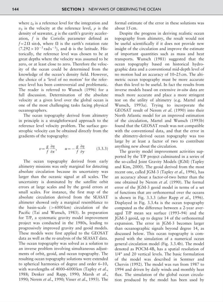
reference level velocity problem. The surface geostrophic velocity can be obtained directly from the
gradients of the topography:
v:
,
u:9
(3.3.3)
The ocean topography derived from early
altimetry missions was only marginal for detecting
absolute circulation because its uncertainty was
larger than the oceanic signal at all scales. The
uncertainty is dominated by the satellite orbit
errors at large scales and by the geoid errors at
small scales. For instance, the first map of the
absolute circulation derived from the SEASAT
altimeter showed only a marginal resemblance to
the basin-scale (96000 km) circulation of the
Pacific (Tai and Wunsch, 1983). In preparation
for T/P, a systematic gravity model improvement
project was conducted in the 1980s, leading to
progressively improved gravity and geoid models.
These models were first applied to the GEOSAT
data as well as the re-analysis of the SEASAT data.
The ocean topography was solved as a solution to
an inverse problem involving simultaneous adjustments of orbit, geoid, and ocean topography. The
resulting ocean topography solutions were extended
to spherical harmonics of degree and order 6–10,
with wavelengths of 4000–6000 km (Tapley et al.,
1988; Denker and Rapp, 1990; Marsh et al.,
1990; Nerem et al., 1990; Visser et al., 1993). The
formal estimate of the error in these solutions was
about 15 cm.
Despite the progress in deriving realistic ocean
topography from altimetry, the result would not
be useful scientifically if it does not provide new
insight of the circulation and improve the estimate
of important quantities such as mass and heat
transports. Wunsch (1981) suggested that the
ocean topography based on historical hydrographic data and a conventional mid-depth level of
no motion had an accuracy of 10–25 cm. The altimetric ocean topography must be more accurate
than this level to be useful. In fact the results from
inverse models based on extensive in-situ data are
much more accurate and place a more stringent
test on the utility of altimetry (e.g. Martel and
Wunsch, 1993a). Trying to incorporate the
GEOSAT result of Nerem et al. (1990) into their
North Atlantic model for an improved estimation
of the circulation, Martel and Wunsch (1993b)
found that the GEOSAT result was not compatible
with the conventional data, and that the error in
the altimetry-derived ocean topography was too
large by at least a factor of two to contribute
anything new about the circulation.
The gravity model improvement activities supported by the T/P project culminated in a series of
the so-called Joint Gravity Models (JGM) (Tapley
and Kim, 2000). The geoid derived from the most
recent one, called JGM-3 (Tapley et al., 1996), has
an accuracy about a factor-of-two better than the
one obtained by Nerem et al. (1990). The formal
error of the JGM-3 geoid model in terms of a set
of functions that are orthonormal over the oceans
is shown in Fig. 3.3.3 (after Rapp et al., 1996).
Displayed in Fig. 3.3.4a is the ocean topography
computed as the difference between a 2-year averaged T/P mean sea surface (1993–94) and the
JGM-3 geoid, up to degree 14 of the orthonormal
expansion. The error in JGM-3 becomes larger
than oceanographic signals beyond degree 14, as
discussed below. This ocean topography is compared with the simulation of a numerical ocean
general circulation model (Fig. 3.3.4b). The model
denoted as POCM-4B, has a spatial resolution of
1/4° and 20 vertical levels. The basic formulation
of the model was described in Semtner and
Chervin (1992). The model was run from 1987 to
1994 and driven by daily winds and monthly heat
flux. The simulation of the global ocean circulation produced by the model has been used by
Ѩ
ᎏ
Ѩy
g
ᎏ
f
Ѩ
ᎏ
Ѩx
g
ᎏ
f
SECTION 3 NEW WAYS OF OBSERVING THE OCEAN
144
v 0 is the velocity at the reference level, is the
density of seawater, g is the earth’s gravity acceleration, f is the Coriolis parameter defined as
f:2 ⍀ sin , where ⍀ is the earth’s rotation rate
(7.29210
95 rad s
91
), and is the latitude. Historically, the reference level was chosen to be at
great depths where the velocity was assumed to be
zero, or at least close to zero. Therefore the velocity of the ocean could be determined from the
knowledge of the ocean’s density field. However,
the choice of a ‘level of no motion’ for the reference level has been controversial and problematic.
The reader is referred to Wunsch (1996) for a
full discussion. Determination of the absolute
velocity at a given level over the global ocean is
one of the most challenging tasks facing physical
oceanographers.
The ocean topography derived from altimetry
in principle is a straightforward approach to the
reference level velocity problem. The surface geostrophic velocity can be obtained directly from the
gradients of the topography:
v:
,
u:9
(3.3.3)
The ocean topography derived from early
altimetry missions was only marginal for detecting
absolute circulation because its uncertainty was
larger than the oceanic signal at all scales. The
uncertainty is dominated by the satellite orbit
errors at large scales and by the geoid errors at
small scales. For instance, the first map of the
absolute circulation derived from the SEASAT
altimeter showed only a marginal resemblance to
the basin-scale (96000 km) circulation of the
Pacific (Tai and Wunsch, 1983). In preparation
for T/P, a systematic gravity model improvement
project was conducted in the 1980s, leading to
progressively improved gravity and geoid models.
These models were first applied to the GEOSAT
data as well as the re-analysis of the SEASAT data.
The ocean topography was solved as a solution to
an inverse problem involving simultaneous adjustments of orbit, geoid, and ocean topography. The
resulting ocean topography solutions were extended
to spherical harmonics of degree and order 6–10,
with wavelengths of 4000–6000 km (Tapley et al.,
1988; Denker and Rapp, 1990; Marsh et al.,
1990; Nerem et al., 1990; Visser et al., 1993). The
formal estimate of the error in these solutions was
about 15 cm.
Despite the progress in deriving realistic ocean
topography from altimetry, the result would not
be useful scientifically if it does not provide new
insight of the circulation and improve the estimate
of important quantities such as mass and heat
transports. Wunsch (1981) suggested that the
ocean topography based on historical hydrographic data and a conventional mid-depth level of
no motion had an accuracy of 10–25 cm. The altimetric ocean topography must be more accurate
than this level to be useful. In fact the results from
inverse models based on extensive in-situ data are
much more accurate and place a more stringent
test on the utility of altimetry (e.g. Martel and
Wunsch, 1993a). Trying to incorporate the
GEOSAT result of Nerem et al. (1990) into their
North Atlantic model for an improved estimation
of the circulation, Martel and Wunsch (1993b)
found that the GEOSAT result was not compatible
with the conventional data, and that the error in
the altimetry-derived ocean topography was too
large by at least a factor of two to contribute
anything new about the circulation.
The gravity model improvement activities supported by the T/P project culminated in a series of
the so-called Joint Gravity Models (JGM) (Tapley
and Kim, 2000). The geoid derived from the most
recent one, called JGM-3 (Tapley et al., 1996), has
an accuracy about a factor-of-two better than the
one obtained by Nerem et al. (1990). The formal
error of the JGM-3 geoid model in terms of a set
of functions that are orthonormal over the oceans
is shown in Fig. 3.3.3 (after Rapp et al., 1996).
Displayed in Fig. 3.3.4a is the ocean topography
computed as the difference between a 2-year averaged T/P mean sea surface (1993–94) and the
JGM-3 geoid, up to degree 14 of the orthonormal
expansion. The error in JGM-3 becomes larger
than oceanographic signals beyond degree 14, as
discussed below. This ocean topography is compared with the simulation of a numerical ocean
general circulation model (Fig. 3.3.4b). The model
denoted as POCM-4B, has a spatial resolution of
1/4° and 20 vertical levels. The basic formulation
of the model was described in Semtner and
Chervin (1992). The model was run from 1987 to
1994 and driven by daily winds and monthly heat
flux. The simulation of the global ocean circulation produced by the model has been used by
Ѩ
ᎏ
Ѩy
g
ᎏ
f
Ѩ
ᎏ
Ѩx
g
ᎏ
f
SECTION 3 NEW WAYS OF OBSERVING THE OCEAN
144