

silicate rocks expressed in moles of divalent ions
(Ca
2þ or Mg
2þ ) per unit of time (i.e., the rates of
reactions [I] and [II]), F CD is the carbonate deposition flux, F OW is the carbon input flux from
weathering-oxidation of crustal organic carbon, and
F OD is the organic carbon deposition flux. Note that
the silicate weathering flux does not appear in the
carbon budget, eqn [4b], since silicate weathering
(reaction [II]) transfers carbon from the atmosphere
to the ocean but does not remove it from the
atmosphere–ocean system. The factor of 2 in eqn
[4a] results from the fact that two equivalents of
alkalinity are transferred to the ocean when one
Ca
2þ or Mg
2þ ion is delivered to the ocean by rivers
(reactions [I] and [II]). The same factor of 2 holds
for carbonate deposition, which is the reverse of reaction [I]. As already mentioned, the atmosphere–
ocean system must be close to equilibrium, so that
the derivatives on the left-hand side of eqns [4a] and
[4b] can be set to zero. This assumption transforms
the differential equation system into a set of two
algebraic equations, which can be solved to yield
eqn [5].
F VOL À F SW ¼ F OD À F OW
½5
This equation leads to eqn [1] if the effect of the
organic subcycle is neglected (i.e., when this subcycle
is set to equilibrium). Hence, eqn [5] is a generalization of the Walker, Hays, and Kasting budget. It
states that the disequilibrium of the inorganic part of
the carbon cycle must be compensated for by a disequilibrium of opposite sign in the organic subcycle.
Use of Isotopic Data (Inverse Modeling)
To solve eqns [4] or [5], some kinetic laws must be
provided for the fluxes, that is, the relations between
these fluxes, time t, and the reservoir contents, or
atmospheric PCO 2 , must be known. Such kinetic laws
are, however, poorly known, so it may be preferable,
at least for some fluxes, to use forcing functions in
the calculation of these fluxes. For example, volcanic
fluxes are often made proportional to the seafloor
spreading rate and weathering fluxes to land area, for
which past reconstructions are available. Ocean
isotopic records, such as those presented earlier, can
also be used to force the model. Budget equations
similar to [2] are then written for the relevant isotopes and transformed into equations containing
isotopic ratios r (or d, the relative departure of the
isotopic ratio from a standard). The sea water
87 Sr/
86 Sr ratio has been used in this way to estimate
the silicate weathering flux F SW , but as discussed
earlier the results are strongly dependent on the hypothesis of constancy for the isotopic ratios of
weathered products. The
13 C isotopic history of the
ocean has been used in many models, since the beginning of the 1980s, to constrain the organic carbon
subcycle. The
13 C isotopic budget for the ocean can
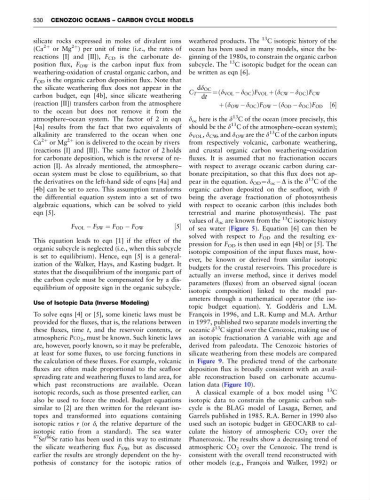
be written as eqn [6].
C T
dd OC
dt
¼ d VOL À d OC
ð
Þ F VOL þ d CW À d OC
ð
Þ F CW
þ d OW À d OC
ð
Þ F OW À d OD À d OC
ð
Þ F OD ½6
d oc here is the d
13 C of the ocean (more precisely, this
should be the d
13
C of the atmosphere–ocean system);
d VOL , d CW , and d OW are the d
13 C of the carbon inputs
from respectively volcanic, carbonate weathering,
and crustal organic carbon weathering–oxidation
fluxes. It is assumed that no fractionation occurs
with respect to average oceanic carbon during carbonate precipitation, so that this flux does not appear in the equation. d OD ¼ d oc À D is the d
13 C of the
organic carbon deposited on the seafloor, with y
being the average fractionation of photosynthesis
with respect to oceanic carbon (this includes both
terrestrial and marine photosynthesis). The past
values of d oc are known from the
13 C isotopic history
of sea water (Figure 5). Equation [6] can then be
solved with respect to F OD and the resulting expression for F OD is then used in eqn [4b] or [5]. The
isotopic composition of the input fluxes must, however, be known or derived from similar isotopic
budgets for the crustal reservoirs. This procedure is
actually an inverse method, since it derives model
parameters (fluxes) from an observed signal (ocean
isotopic composition) linked to the model parameters through a mathematical operator (the isotopic budget equation). Y. Godde ´ris and L.M.
Franc¸ ois in 1996, and L.R. Kump and M.A. Arthur
in 1997, published two separate models inverting the
oceanic d
13
C signal over the Cenozoic, making use of
an isotopic fractionation D variable with age and
derived from paleodata. The Cenozoic histories of
silicate weathering from these models are compared
in Figure 9. The predicted trend of the carbonate
deposition flux is broadly consistent with an available reconstruction based on carbonate accumulation data (Figure 10).
A classical example of a box model using
13
C
isotopic data to constrain the organic carbon subcycle is the BLAG model of Lasaga, Berner, and
Garrels published in 1985. R.A. Berner in 1990 also
used such an isotopic budget in GEOCARB to calculate the history of atmospheric CO 2 over the
Phanerozoic. The results show a decreasing trend of
atmospheric CO 2 over the Cenozoic. The trend is
consistent with the overall trend reconstructed with
other models (e.g., Franc¸ ois and Walker, 1992) or
530 CENOZOIC OCEANS – CARBON CYCLE MODELS
(Ca
2þ or Mg
2þ ) per unit of time (i.e., the rates of
reactions [I] and [II]), F CD is the carbonate deposition flux, F OW is the carbon input flux from
weathering-oxidation of crustal organic carbon, and
F OD is the organic carbon deposition flux. Note that
the silicate weathering flux does not appear in the
carbon budget, eqn [4b], since silicate weathering
(reaction [II]) transfers carbon from the atmosphere
to the ocean but does not remove it from the
atmosphere–ocean system. The factor of 2 in eqn
[4a] results from the fact that two equivalents of
alkalinity are transferred to the ocean when one
Ca
2þ or Mg
2þ ion is delivered to the ocean by rivers
(reactions [I] and [II]). The same factor of 2 holds
for carbonate deposition, which is the reverse of reaction [I]. As already mentioned, the atmosphere–
ocean system must be close to equilibrium, so that
the derivatives on the left-hand side of eqns [4a] and
[4b] can be set to zero. This assumption transforms
the differential equation system into a set of two
algebraic equations, which can be solved to yield
eqn [5].
F VOL À F SW ¼ F OD À F OW
½5
This equation leads to eqn [1] if the effect of the
organic subcycle is neglected (i.e., when this subcycle
is set to equilibrium). Hence, eqn [5] is a generalization of the Walker, Hays, and Kasting budget. It
states that the disequilibrium of the inorganic part of
the carbon cycle must be compensated for by a disequilibrium of opposite sign in the organic subcycle.
Use of Isotopic Data (Inverse Modeling)
To solve eqns [4] or [5], some kinetic laws must be
provided for the fluxes, that is, the relations between
these fluxes, time t, and the reservoir contents, or
atmospheric PCO 2 , must be known. Such kinetic laws
are, however, poorly known, so it may be preferable,
at least for some fluxes, to use forcing functions in
the calculation of these fluxes. For example, volcanic
fluxes are often made proportional to the seafloor
spreading rate and weathering fluxes to land area, for
which past reconstructions are available. Ocean
isotopic records, such as those presented earlier, can
also be used to force the model. Budget equations
similar to [2] are then written for the relevant isotopes and transformed into equations containing
isotopic ratios r (or d, the relative departure of the
isotopic ratio from a standard). The sea water
87 Sr/
86 Sr ratio has been used in this way to estimate
the silicate weathering flux F SW , but as discussed
earlier the results are strongly dependent on the hypothesis of constancy for the isotopic ratios of
weathered products. The
13 C isotopic history of the
ocean has been used in many models, since the beginning of the 1980s, to constrain the organic carbon
subcycle. The
13 C isotopic budget for the ocean can
be written as eqn [6].
C T
dd OC
dt
¼ d VOL À d OC
ð
Þ F VOL þ d CW À d OC
ð
Þ F CW
þ d OW À d OC
ð
Þ F OW À d OD À d OC
ð
Þ F OD ½6
d oc here is the d
13 C of the ocean (more precisely, this
should be the d
13
C of the atmosphere–ocean system);
d VOL , d CW , and d OW are the d
13 C of the carbon inputs
from respectively volcanic, carbonate weathering,
and crustal organic carbon weathering–oxidation
fluxes. It is assumed that no fractionation occurs
with respect to average oceanic carbon during carbonate precipitation, so that this flux does not appear in the equation. d OD ¼ d oc À D is the d
13 C of the
organic carbon deposited on the seafloor, with y
being the average fractionation of photosynthesis
with respect to oceanic carbon (this includes both
terrestrial and marine photosynthesis). The past
values of d oc are known from the
13 C isotopic history
of sea water (Figure 5). Equation [6] can then be
solved with respect to F OD and the resulting expression for F OD is then used in eqn [4b] or [5]. The
isotopic composition of the input fluxes must, however, be known or derived from similar isotopic
budgets for the crustal reservoirs. This procedure is
actually an inverse method, since it derives model
parameters (fluxes) from an observed signal (ocean
isotopic composition) linked to the model parameters through a mathematical operator (the isotopic budget equation). Y. Godde ´ris and L.M.
Franc¸ ois in 1996, and L.R. Kump and M.A. Arthur
in 1997, published two separate models inverting the
oceanic d
13
C signal over the Cenozoic, making use of
an isotopic fractionation D variable with age and
derived from paleodata. The Cenozoic histories of
silicate weathering from these models are compared
in Figure 9. The predicted trend of the carbonate
deposition flux is broadly consistent with an available reconstruction based on carbonate accumulation data (Figure 10).
A classical example of a box model using
13
C
isotopic data to constrain the organic carbon subcycle is the BLAG model of Lasaga, Berner, and
Garrels published in 1985. R.A. Berner in 1990 also
used such an isotopic budget in GEOCARB to calculate the history of atmospheric CO 2 over the
Phanerozoic. The results show a decreasing trend of
atmospheric CO 2 over the Cenozoic. The trend is
consistent with the overall trend reconstructed with
other models (e.g., Franc¸ ois and Walker, 1992) or
530 CENOZOIC OCEANS – CARBON CYCLE MODELS