

depending on the availability of nutrients, among
which phosphorus is thought to play a key role. The
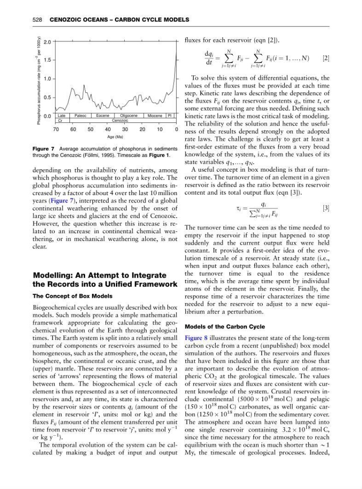
global phosphorus accumulation into sediments increased by a factor of about 4 over the last 10 million
years (Figure 7), interpreted as the record of a global
continental weathering enhanced by the onset of
large ice sheets and glaciers at the end of Cenozoic.
However, the question whether this increase is related to an increase in continental chemical weathering, or in mechanical weathering alone, is not
clear.
Modelling: An Attempt to Integrate
the Records into a Unified Framework
The Concept of Box Models
Biogeochemical cycles are usually described with box
models. Such models provide a simple mathematical
framework appropriate for calculating the geochemical evolution of the Earth through geological
times. The Earth system is split into a relatively small
number of components or reservoirs assumed to be
homogeneous, such as the atmosphere, the ocean, the
biosphere, the continental or oceanic crust, and the
(upper) mantle. These reservoirs are connected by a
series of ‘arrows’ representing the flows of material
between them. The biogeochemical cycle of each
element is thus represented as a set of interconnected
reservoirs and, at any time, its state is characterized
by the reservoir sizes or contents q i (amount of the
element in reservoir ‘I’, units: mol or kg) and the
fluxes F ij (amount of the element transferred per unit
time from reservoir ‘I’ to reservoir ‘j’, units: mol y
À1
or kg y
À1 ).
The temporal evolution of the system can be calculated by making a budget of input and output
fluxes for each reservoir (eqn [2]).
dq i
dt
¼
X N
j¼1jai
F ji À
X N
j¼1jai
F ij i ¼ 1; y; N
ð
Þ
½ 2
To solve this system of differential equations, the
values of the fluxes must be provided at each time
step. Kinetic rate laws describing the dependence of
the fluxes F ij on the reservoir contents q i , time t, or
some external forcing are thus needed. Defining such
kinetic rate laws is the most critical task of modeling.
The reliability of the solution and hence the usefulness of the results depend strongly on the adopted
rate laws. The challenge is clearly to get at least a
first-order estimate of the fluxes from a very broad
knowledge of the system, i.e., from the values of its
state variables q 1 ,y, q N .
A useful concept in box modeling is that of turnover time. The turnover time of an element in a given
reservoir is defined as the ratio between its reservoir
content and its total output flux (eqn [3]).
t i ¼
q i
P N
j¼1jai F ij
½3
The turnover time can be seen as the time needed to
empty the reservoir if the input happened to stop
suddenly and the current output flux were held
constant. It provides a first-order idea of the evolution timescale of a reservoir. At steady state (i.e.,
when input and output fluxes balance each other),
the turnover time is equal to the residence
time, which is the average time spent by individual
atoms of the element in the reservoir. Finally, the
response time of a reservoir characterizes the time
needed for the reservoir to adjust to a new equilibrium after a perturbation.
Models of the Carbon Cycle
Figure 8 illustrates the present state of the long-term
carbon cycle from a recent (unpublished) box model
simulation of the authors. The reservoirs and fluxes
that have been included in this figure are those that
are important to describe the evolution of atmospheric CO 2 at the geological timescale. The values
of reservoir sizes and fluxes are consistent with current knowledge of the system. Crustal reservoirs include continental (5000 Â 10
18 mol C) and pelagic
(150 Â 10
18 mol C) carbonates, as well organic carbon (1250 Â 10
18 mol C) from the sedimentary cover.
The atmosphere and ocean have been lumped into
one single reservoir containing 3.2 Â 10
18 mol C,
since the time necessary for the atmosphere to reach
equilibrium with the ocean is much shorter than B1
My, the timescale of geological processes. Indeed,
70
60
50
40
30
20
10
0
Age (Ma)
0.0
0.5
1.0
1.5
2.0
Cr
Cenozoic
Late
Eocene
Miocene Pl
Paleoc
Oligocene
Phosphorus accumulation rate (mg cm
_
2
per 1000 y)
Figure 7 Average accumulation of phosphorus in sediments
through the Cenozoic (Fo ¨ llmi, 1995). Timescale as Figure 1.
528 CENOZOIC OCEANS – CARBON CYCLE MODELS
which phosphorus is thought to play a key role. The
global phosphorus accumulation into sediments increased by a factor of about 4 over the last 10 million
years (Figure 7), interpreted as the record of a global
continental weathering enhanced by the onset of
large ice sheets and glaciers at the end of Cenozoic.
However, the question whether this increase is related to an increase in continental chemical weathering, or in mechanical weathering alone, is not
clear.
Modelling: An Attempt to Integrate
the Records into a Unified Framework
The Concept of Box Models
Biogeochemical cycles are usually described with box
models. Such models provide a simple mathematical
framework appropriate for calculating the geochemical evolution of the Earth through geological
times. The Earth system is split into a relatively small
number of components or reservoirs assumed to be
homogeneous, such as the atmosphere, the ocean, the
biosphere, the continental or oceanic crust, and the
(upper) mantle. These reservoirs are connected by a
series of ‘arrows’ representing the flows of material
between them. The biogeochemical cycle of each
element is thus represented as a set of interconnected
reservoirs and, at any time, its state is characterized
by the reservoir sizes or contents q i (amount of the
element in reservoir ‘I’, units: mol or kg) and the
fluxes F ij (amount of the element transferred per unit
time from reservoir ‘I’ to reservoir ‘j’, units: mol y
À1
or kg y
À1 ).
The temporal evolution of the system can be calculated by making a budget of input and output
fluxes for each reservoir (eqn [2]).
dq i
dt
¼
X N
j¼1jai
F ji À
X N
j¼1jai
F ij i ¼ 1; y; N
ð
Þ
½ 2
To solve this system of differential equations, the
values of the fluxes must be provided at each time
step. Kinetic rate laws describing the dependence of
the fluxes F ij on the reservoir contents q i , time t, or
some external forcing are thus needed. Defining such
kinetic rate laws is the most critical task of modeling.
The reliability of the solution and hence the usefulness of the results depend strongly on the adopted
rate laws. The challenge is clearly to get at least a
first-order estimate of the fluxes from a very broad
knowledge of the system, i.e., from the values of its
state variables q 1 ,y, q N .
A useful concept in box modeling is that of turnover time. The turnover time of an element in a given
reservoir is defined as the ratio between its reservoir
content and its total output flux (eqn [3]).
t i ¼
q i
P N
j¼1jai F ij
½3
The turnover time can be seen as the time needed to
empty the reservoir if the input happened to stop
suddenly and the current output flux were held
constant. It provides a first-order idea of the evolution timescale of a reservoir. At steady state (i.e.,
when input and output fluxes balance each other),
the turnover time is equal to the residence
time, which is the average time spent by individual
atoms of the element in the reservoir. Finally, the
response time of a reservoir characterizes the time
needed for the reservoir to adjust to a new equilibrium after a perturbation.
Models of the Carbon Cycle
Figure 8 illustrates the present state of the long-term
carbon cycle from a recent (unpublished) box model
simulation of the authors. The reservoirs and fluxes
that have been included in this figure are those that
are important to describe the evolution of atmospheric CO 2 at the geological timescale. The values
of reservoir sizes and fluxes are consistent with current knowledge of the system. Crustal reservoirs include continental (5000 Â 10
18 mol C) and pelagic
(150 Â 10
18 mol C) carbonates, as well organic carbon (1250 Â 10
18 mol C) from the sedimentary cover.
The atmosphere and ocean have been lumped into
one single reservoir containing 3.2 Â 10
18 mol C,
since the time necessary for the atmosphere to reach
equilibrium with the ocean is much shorter than B1
My, the timescale of geological processes. Indeed,
70
60
50
40
30
20
10
0
Age (Ma)
0.0
0.5
1.0
1.5
2.0
Cr
Cenozoic
Late
Eocene
Miocene Pl
Paleoc
Oligocene
Phosphorus accumulation rate (mg cm
_
2
per 1000 y)
Figure 7 Average accumulation of phosphorus in sediments
through the Cenozoic (Fo ¨ llmi, 1995). Timescale as Figure 1.
528 CENOZOIC OCEANS – CARBON CYCLE MODELS