

This form of modeling, however, is particularly useful for describing regional patterns and in the areas
where simple tracer age approaches breakdown.
Three-Dimensional (3-D) Biogeochemical
Simulations
By their very nature, idealized models neglect many
important aspects of ocean dynamics. The alternative
is full 3-D ocean GCMs, which incorporate more
realistic spatial and temporal geometry and a much
fuller suite of physics. There are several different
families of ocean physical models characterized by
the underlying governing equations and the vertical
discretization schemes. Within model families, individual simulations will differ in important factors of
surface forcing and choice of physical parametrizations. Often these parametrizations account for
complex processes, such as turbulent mixing, that
occur on small space scales that are not directly resolved or computed by the model but which can have
important impacts on the larger-scale ocean circulation; often an exact description of specific events is
not required and a statistical representation of these
subgrid scale processes is sufficient. For example,
turbulent mixing is commonly treated using equations analogous to those for Fickian molecular diffusion. Ocean GCMs, particularly coarse-resolution
global versions, are sensitive to the subgrid scale
parametrizations used to account for unresolved
processes such as mesoscale eddy mixing, surface and
bottom boundary layer dynamics, and air–sea and
ocean–ice interactions. Different models will be better or worse for different biogeochemical problems.
Considerable progress has been achieved over the
last two decades on the incorporation of chemical
tracers, biogeochemistry, and ecosystem dynamics
into both regional and global 3-D models. Modeling
groups now routinely simulate the more commonly
measured tracers (e.g., radiocarbon, chlorofluorocarbons, and tritium–
3
He). Most of these tracers
have surface sources and, therefore, provide clear
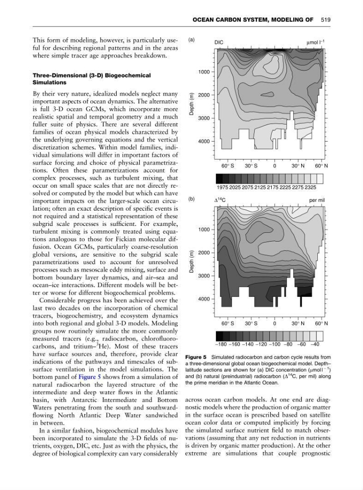
indications of the pathways and timescales of subsurface ventilation in the model simulations. The
bottom panel of Figure 5 shows from a simulation of
natural radiocarbon the layered structure of the
intermediate and deep water flows in the Atlantic
basin, with Antarctic Intermediate and Bottom
Waters penetrating from the south and southwardflowing North Atlantic Deep Water sandwiched
in between.
In a similar fashion, biogeochemical modules have
been incorporated to simulate the 3-D fields of nutrients, oxygen, DIC, etc. Just as with the physics, the
degree of biological complexity can vary considerably
across ocean carbon models. At one end are diagnostic models where the production of organic matter
in the surface ocean is prescribed based on satellite
ocean color data or computed implicitly by forcing
the simulated surface nutrient field to match observations (assuming that any net reduction in nutrients
is driven by organic matter production). At the other
extreme are simulations that couple prognostic
1000
2000
3000
4000
Depth (m)
60° S
30° S
0
3 0 ° N
60° N
1000
2000
3000
4000
Depth (m)
60° S
30° S
0
3 0 ° N
60° N
1975 2025 2075 2125 2175 2225 2275 2325
−180 −160 −140 −120 −100 −80 −60 −40
DIC
μmol l −1
Δ 14 C
per mil
(b)
(a)
Figure 5 Simulated radiocarbon and carbon cycle results from
a three-dimensional global ocean biogeochemical model. Depth–
latitude sections are shown for (a) DIC concentration (mmol l
À 1
)
and (b) natural (preindustrial) radiocarbon (D
14
C, per mil) along
the prime meridian in the Atlantic Ocean.
OCEAN CARBON SYSTEM, MODELING OF 519
where simple tracer age approaches breakdown.
Three-Dimensional (3-D) Biogeochemical
Simulations
By their very nature, idealized models neglect many
important aspects of ocean dynamics. The alternative
is full 3-D ocean GCMs, which incorporate more
realistic spatial and temporal geometry and a much
fuller suite of physics. There are several different
families of ocean physical models characterized by
the underlying governing equations and the vertical
discretization schemes. Within model families, individual simulations will differ in important factors of
surface forcing and choice of physical parametrizations. Often these parametrizations account for
complex processes, such as turbulent mixing, that
occur on small space scales that are not directly resolved or computed by the model but which can have
important impacts on the larger-scale ocean circulation; often an exact description of specific events is
not required and a statistical representation of these
subgrid scale processes is sufficient. For example,
turbulent mixing is commonly treated using equations analogous to those for Fickian molecular diffusion. Ocean GCMs, particularly coarse-resolution
global versions, are sensitive to the subgrid scale
parametrizations used to account for unresolved
processes such as mesoscale eddy mixing, surface and
bottom boundary layer dynamics, and air–sea and
ocean–ice interactions. Different models will be better or worse for different biogeochemical problems.
Considerable progress has been achieved over the
last two decades on the incorporation of chemical
tracers, biogeochemistry, and ecosystem dynamics
into both regional and global 3-D models. Modeling
groups now routinely simulate the more commonly
measured tracers (e.g., radiocarbon, chlorofluorocarbons, and tritium–
3
He). Most of these tracers
have surface sources and, therefore, provide clear
indications of the pathways and timescales of subsurface ventilation in the model simulations. The
bottom panel of Figure 5 shows from a simulation of
natural radiocarbon the layered structure of the
intermediate and deep water flows in the Atlantic
basin, with Antarctic Intermediate and Bottom
Waters penetrating from the south and southwardflowing North Atlantic Deep Water sandwiched
in between.
In a similar fashion, biogeochemical modules have
been incorporated to simulate the 3-D fields of nutrients, oxygen, DIC, etc. Just as with the physics, the
degree of biological complexity can vary considerably
across ocean carbon models. At one end are diagnostic models where the production of organic matter
in the surface ocean is prescribed based on satellite
ocean color data or computed implicitly by forcing
the simulated surface nutrient field to match observations (assuming that any net reduction in nutrients
is driven by organic matter production). At the other
extreme are simulations that couple prognostic
1000
2000
3000
4000
Depth (m)
60° S
30° S
0
3 0 ° N
60° N
1000
2000
3000
4000
Depth (m)
60° S
30° S
0
3 0 ° N
60° N
1975 2025 2075 2125 2175 2225 2275 2325
−180 −160 −140 −120 −100 −80 −60 −40
DIC
μmol l −1
Δ 14 C
per mil
(b)
(a)
Figure 5 Simulated radiocarbon and carbon cycle results from
a three-dimensional global ocean biogeochemical model. Depth–
latitude sections are shown for (a) DIC concentration (mmol l
À 1
)
and (b) natural (preindustrial) radiocarbon (D
14
C, per mil) along
the prime meridian in the Atlantic Ocean.
OCEAN CARBON SYSTEM, MODELING OF 519