

treatments of multiple phytoplankton, zooplankton,
and bacteria species to the biogeochemical tracers.
Transient tracers enter the picture because the biogeochemical distributions are also strongly influenced
circulation. This is nicely illustrated by comparing
the simulated radiocarbon and DIC sections in
Figure 5. To first order, older waters marked by low
radiocarbon exhibit high DIC levels due to the
accumulation of carbon released from particle remineralization. Tracers can be used to guide the improvement of the physical circulation and highlight
areas where the circulation is poor and thus the
biogeochemical tracers may be suspect. They can also
be used more quantitatively to create model skill
metrics; this approach can be applied across multiple
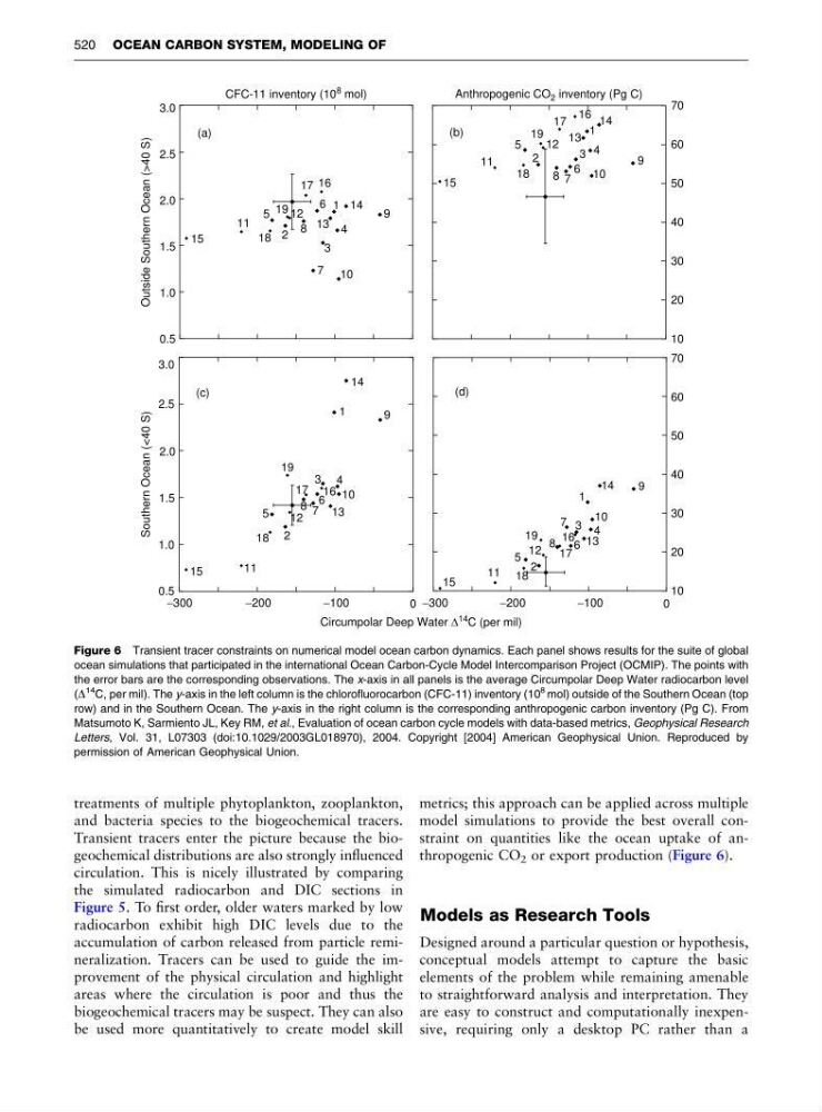
model simulations to provide the best overall constraint on quantities like the ocean uptake of anthropogenic CO 2 or export production (Figure 6).
Models as Research Tools
Designed around a particular question or hypothesis,
conceptual models attempt to capture the basic
elements of the problem while remaining amenable
to straightforward analysis and interpretation. They
are easy to construct and computationally inexpensive, requiring only a desktop PC rather than a
−300
−200
−100
0
Circumpolar Deep Water Δ 14 C (per mil)
−300
−200
−100
0
CFC-11 inventory (10
8 mol)
Anthropogenic CO 2 inventory (Pg C)
Southern Ocean (<40 S)
10
20
30
40
50
60
70
Outside Southern Ocean (>40 S)
1
9
7
14
3
5
11
12
13
4
8
2
10
15
16
19
18
6
17
1
9
7
14
3
5
11
12
13 4
8
2
10
15
17 16
19
18
6
10
20
30
40
50
60
70
0.5
1.0
1.5
2.0
2.5
3.0
0.5
1.0
1.5
2.0
2.5
3.0
1
9
7
14
3
5
11
12
13
4
8
2
10
15
16
19
18
6
17
1
9
7
14
3
5
11
12
13
4
8
2
10
15
17
16
19
18
6
(c)
(a)
(d)
(b)
Figure 6 Transient tracer constraints on numerical model ocean carbon dynamics. Each panel shows results for the suite of global
ocean simulations that participated in the international Ocean Carbon-Cycle Model Intercomparison Project (OCMIP). The points with
the error bars are the corresponding observations. The x-axis in all panels is the average Circumpolar Deep Water radiocarbon level
(D
14
C, per mil). The y-axis in the left column is the chlorofluorocarbon (CFC-11) inventory (10
8 mol) outside of the Southern Ocean (top
row) and in the Southern Ocean. The y-axis in the right column is the corresponding anthropogenic carbon inventory (Pg C). From
Matsumoto K, Sarmiento JL, Key RM, et al., Evaluation of ocean carbon cycle models with data-based metrics, Geophysical Research
Letters, Vol. 31, L07303 (doi:10.1029/2003GL018970), 2004. Copyright [2004] American Geophysical Union. Reproduced by
permission of American Geophysical Union.
520 OCEAN CARBON SYSTEM, MODELING OF
and bacteria species to the biogeochemical tracers.
Transient tracers enter the picture because the biogeochemical distributions are also strongly influenced
circulation. This is nicely illustrated by comparing
the simulated radiocarbon and DIC sections in
Figure 5. To first order, older waters marked by low
radiocarbon exhibit high DIC levels due to the
accumulation of carbon released from particle remineralization. Tracers can be used to guide the improvement of the physical circulation and highlight
areas where the circulation is poor and thus the
biogeochemical tracers may be suspect. They can also
be used more quantitatively to create model skill
metrics; this approach can be applied across multiple
model simulations to provide the best overall constraint on quantities like the ocean uptake of anthropogenic CO 2 or export production (Figure 6).
Models as Research Tools
Designed around a particular question or hypothesis,
conceptual models attempt to capture the basic
elements of the problem while remaining amenable
to straightforward analysis and interpretation. They
are easy to construct and computationally inexpensive, requiring only a desktop PC rather than a
−300
−200
−100
0
Circumpolar Deep Water Δ 14 C (per mil)
−300
−200
−100
0
CFC-11 inventory (10
8 mol)
Anthropogenic CO 2 inventory (Pg C)
Southern Ocean (<40 S)
10
20
30
40
50
60
70
Outside Southern Ocean (>40 S)
1
9
7
14
3
5
11
12
13
4
8
2
10
15
16
19
18
6
17
1
9
7
14
3
5
11
12
13 4
8
2
10
15
17 16
19
18
6
10
20
30
40
50
60
70
0.5
1.0
1.5
2.0
2.5
3.0
0.5
1.0
1.5
2.0
2.5
3.0
1
9
7
14
3
5
11
12
13
4
8
2
10
15
16
19
18
6
17
1
9
7
14
3
5
11
12
13
4
8
2
10
15
17
16
19
18
6
(c)
(a)
(d)
(b)
Figure 6 Transient tracer constraints on numerical model ocean carbon dynamics. Each panel shows results for the suite of global
ocean simulations that participated in the international Ocean Carbon-Cycle Model Intercomparison Project (OCMIP). The points with
the error bars are the corresponding observations. The x-axis in all panels is the average Circumpolar Deep Water radiocarbon level
(D
14
C, per mil). The y-axis in the left column is the chlorofluorocarbon (CFC-11) inventory (10
8 mol) outside of the Southern Ocean (top
row) and in the Southern Ocean. The y-axis in the right column is the corresponding anthropogenic carbon inventory (Pg C). From
Matsumoto K, Sarmiento JL, Key RM, et al., Evaluation of ocean carbon cycle models with data-based metrics, Geophysical Research
Letters, Vol. 31, L07303 (doi:10.1029/2003GL018970), 2004. Copyright [2004] American Geophysical Union. Reproduced by
permission of American Geophysical Union.
520 OCEAN CARBON SYSTEM, MODELING OF