

carbon between the ocean and atmosphere can occur
only where this close coupling of the carbon and
nutrient cycles breaks down. When subsurface water
is brought to the surface at low latitude, production
draws the nutrients down to near zero and removes
to first order all of the excess seawater DIC and
pCO 2 . Modifications in the upward nutrient flux to
the low latitudes have relatively little impact on the
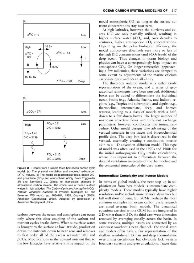
model atmospheric CO 2 as long as the surface nutrient concentrations stay near zero.
At high latitudes, however, the nutrients and excess DIC are only partially utilized, resulting in
higher surface water pCO 2 and, over decades to
centuries, higher atmospheric CO 2 concentrations.
Depending on the polar biological efficiency, the
model atmosphere effectively sees more or less of
the high DIC concentrations (and pCO 2 levels) of the
deep ocean. Thus changes in ocean biology and
physics can have a correspondingly large impact on
atmospheric CO 2 . On longer timescales (approaching a few millennia), these variations are damped to
some extent by adjustments of the marine calcium
carbonate cycle and ocean alkalinity.
The three-box outcrop model is a rather crude
representation of the ocean, and a series of geographical refinements have been pursued. Additional
boxes can be added to differentiate the individual
ocean basins (e.g., Atlantic, Pacific, and Indian), regions (e.g., Tropics and subtropics), and depths (e.g.,
thermocline, intermediate, deep, and bottom
waters), leading to a class of models with a halfdozen to a few dozen boxes. The larger number of
unknown advective flows and turbulent exchange
parameters, however, complicates the tuning procedure. Other model designs take advantage of the
vertical structure in the tracer and biogeochemical
profile data. The deep box (es) is discretized in the
vertical, essentially creating a continuous interior
akin to a 1-D advection–diffusion model. This type
of model was often used in the 1970s and 1980s for
the initial anthropogenic CO 2 uptake calculations,
where it is important to differentiate between the
decadal ventilation timescales of the thermocline and
the centennial timescales of the deep water.
Intermediate Complexity and Inverse Models
In terms of global models, the next step up in sophistication from box models is intermediate complexity models. These models typically have higher
resolution and/or include more physical dynamics but
fall well short of being full GCMs. Perhaps the most
common examples for ocean carbon cycle research
are zonal average basin models. The dynamical
equations are similar to a GCM but are integrated in
2-D rather than in 3-D, the third east–west dimension
removed by averaging zonally across the basin. In
some versions, multiple basins are connected by an
east–west Southern Ocean channel. The zonal average models often have a fair representation of the
shallow wind-driven Ekman and deep thermohaline
overturning circulations but obviously lack western
boundary currents and gyre circulations. Tracer data
Atm.
Atm.
High
High
Low
Low
Deep
Deep
10 Sv
1
19 Sv
45−60 Sv
Δ 14 C = −178
Δ 14 C = −2
Δ
14 C =
−105
Δ 14 C = −54
p CO 2 = 271
PO 4 = 0.2
DIC = 1932
PO 4 = 2.15
DIC = 2256
PO 4 = 1.42
DIC = 2139
(a)
(b)
Figure 3 Results from a simple three-box ocean carbon cycle
model. (a) The physical circulation and modeled radiocarbon
(D
14
C) values. (b) The model biogeochemical fields, ocean DIC,
and phosphate (PO 4 ) and atmospheric pCO 2 . From Toggweiler
JR and Sarmiento JL, Glacial to inter-glacial changes in
atmospheric carbon dioxide: The critical role of ocean surface
waters in high latitudes, The Carbon Cycle and Atmospheric CO 2 :
Natural Variations Archean to Present, Sundquist ET and
Broecker WS (eds.), pp. 163–184, 1985, Copyright [1985].
American Geophysical Union. Adapted by permission of
American Geophysical Union.
OCEAN CARBON SYSTEM, MODELING OF 517
only where this close coupling of the carbon and
nutrient cycles breaks down. When subsurface water
is brought to the surface at low latitude, production
draws the nutrients down to near zero and removes
to first order all of the excess seawater DIC and
pCO 2 . Modifications in the upward nutrient flux to
the low latitudes have relatively little impact on the
model atmospheric CO 2 as long as the surface nutrient concentrations stay near zero.
At high latitudes, however, the nutrients and excess DIC are only partially utilized, resulting in
higher surface water pCO 2 and, over decades to
centuries, higher atmospheric CO 2 concentrations.
Depending on the polar biological efficiency, the
model atmosphere effectively sees more or less of
the high DIC concentrations (and pCO 2 levels) of the
deep ocean. Thus changes in ocean biology and
physics can have a correspondingly large impact on
atmospheric CO 2 . On longer timescales (approaching a few millennia), these variations are damped to
some extent by adjustments of the marine calcium
carbonate cycle and ocean alkalinity.
The three-box outcrop model is a rather crude
representation of the ocean, and a series of geographical refinements have been pursued. Additional
boxes can be added to differentiate the individual
ocean basins (e.g., Atlantic, Pacific, and Indian), regions (e.g., Tropics and subtropics), and depths (e.g.,
thermocline, intermediate, deep, and bottom
waters), leading to a class of models with a halfdozen to a few dozen boxes. The larger number of
unknown advective flows and turbulent exchange
parameters, however, complicates the tuning procedure. Other model designs take advantage of the
vertical structure in the tracer and biogeochemical
profile data. The deep box (es) is discretized in the
vertical, essentially creating a continuous interior
akin to a 1-D advection–diffusion model. This type
of model was often used in the 1970s and 1980s for
the initial anthropogenic CO 2 uptake calculations,
where it is important to differentiate between the
decadal ventilation timescales of the thermocline and
the centennial timescales of the deep water.
Intermediate Complexity and Inverse Models
In terms of global models, the next step up in sophistication from box models is intermediate complexity models. These models typically have higher
resolution and/or include more physical dynamics but
fall well short of being full GCMs. Perhaps the most
common examples for ocean carbon cycle research
are zonal average basin models. The dynamical
equations are similar to a GCM but are integrated in
2-D rather than in 3-D, the third east–west dimension
removed by averaging zonally across the basin. In
some versions, multiple basins are connected by an
east–west Southern Ocean channel. The zonal average models often have a fair representation of the
shallow wind-driven Ekman and deep thermohaline
overturning circulations but obviously lack western
boundary currents and gyre circulations. Tracer data
Atm.
Atm.
High
High
Low
Low
Deep
Deep
10 Sv
1
19 Sv
45−60 Sv
Δ 14 C = −178
Δ 14 C = −2
Δ
14 C =
−105
Δ 14 C = −54
p CO 2 = 271
PO 4 = 0.2
DIC = 1932
PO 4 = 2.15
DIC = 2256
PO 4 = 1.42
DIC = 2139
(a)
(b)
Figure 3 Results from a simple three-box ocean carbon cycle
model. (a) The physical circulation and modeled radiocarbon
(D
14
C) values. (b) The model biogeochemical fields, ocean DIC,
and phosphate (PO 4 ) and atmospheric pCO 2 . From Toggweiler
JR and Sarmiento JL, Glacial to inter-glacial changes in
atmospheric carbon dioxide: The critical role of ocean surface
waters in high latitudes, The Carbon Cycle and Atmospheric CO 2 :
Natural Variations Archean to Present, Sundquist ET and
Broecker WS (eds.), pp. 163–184, 1985, Copyright [1985].
American Geophysical Union. Adapted by permission of
American Geophysical Union.
OCEAN CARBON SYSTEM, MODELING OF 517