

both fresh and saline groundwater and are ultimately
important in controlling the submarine discharge of
both fluids.
The analysis of coastal groundwater flow must
account for the presence of both fresh- and saline
water components. When appropriate, such as in
regional-scale analysis or for coarse estimation purposes, an assumption can be made that there is a
sharp transition, or interface, between the fresh and
saline groundwater. While this assumption is not
strictly true, it is often appropriate, and invoking it
results in simplifying the analysis. For example, we
can estimate the position of the freshwater–saltwater
interface by assuming a sharp interface, no flow
within the saltwater region, and only horizontal flow
within the fresh groundwater. Invoking these assumptions means that the pressures at adjacent
points along the interface on both the freshwater and
saltwater sides are equal. Equating these pressures
and rearranging, the depth to the interface can be
calculated as follows:
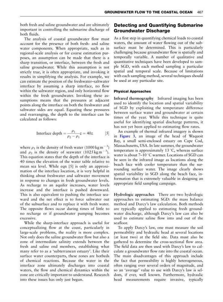
Interface depth ¼
r 1
r 2 À r 1
z ¼ 40z
½5
where r 1 is the density of fresh water (1000 kg m
À 3 )
and r 2 is the density of seawater (1025 kg m
À 3 ).
This equation states that the depth of the interface is
40 times the elevation of the water table relative to
mean sea level. While eqn [5] is only an approximation of the interface location, it is very helpful in
thinking about freshwater and saltwater movement
in response to changes in fresh groundwater levels.
As recharge to an aquifer increases, water levels
increase and the interface is pushed downward.
This is also equivalent to pushing the interface seaward and the net effect is to force saltwater out
of the subsurface and to replace it with fresh water.
The opposite flows occur during times of little to
no recharge or if groundwater pumping becomes
excessive.
While the sharp-interface approach is useful for
conceptualizing flow at the coast, particularly in
large-scale problems, the reality is more complex.
Not only does the saline groundwater flow but also a
zone of intermediate salinity extends between the
fresh and saline end members, establishing what
many refer to as a ‘subterranean estuary’. Like their
surface water counterparts, these zones are hotbeds
of chemical reactions. Because the water in the
interface zone ultimately discharges into coastal
waters, the flow and chemical dynamics within the
zone are critically important to understand. Research
into these issues has only just begun.
Detecting and Quantifying Submarine
Groundwater Discharge
As a first step in quantifying chemical loads to coastal
waters, the amount of water flowing out of the subsurface must be determined. This is particularly
challenging because groundwater flow is spatially and
temporally variable. A number of qualitative and
quantitative techniques have been developed to sample SGD, with each method sampling a particular
spatial and temporal scale. Because of limitations
with each sampling method, several techniques should
be used at any particular site.
Physical Approaches
Infrared thermography Infrared imaging has been
used to identify the location and spatial variability
of SGD by exploiting the temperature difference
between surface water and groundwater at certain
times of the year. While this technique is quite
useful for identifying spatial discharge patterns, it
has not yet been applied to estimating flow rates.
An example of thermal infrared imagery is shown
in Figure 3, an image of the head of Waquoit
Bay, a small semi-enclosed estuary on Cape Cod,
Massachusetts, USA. In late summer, the groundwater
temperature is approximately 13 1C, whereas surface
water is about 7–10 1C warmer. Locations of SGD can
be seen in the infrared image as locations along the
beach face with cooler temperature than the surrounding surface water. The image clearly shows
spatial variability in SGD along the beach face, information that is extremely valuable in designing an
appropriate field sampling campaign.
Hydrologic approaches There are two hydrologic
approaches to estimating SGD: the mass balance
method and Darcy’s law calculation. Both methods
are typically applied to estimating fresh groundwater discharge, although Darcy’s law can also be
used to estimate saline flow into and out of the
seafloor.
To apply Darcy’s law, one must measure the soil
permeability and hydraulic head at several locations
(at least two) at the field site. Data must also be
gathered to determine the cross-sectional flow area.
The field data are then used with Darcy’s law to calculate a groundwater flow rate into the coastal ocean.
The main disadvantages of this approach include
the fact that permeability is highly heterogeneous,
often ranging over several orders of magnitude, and
so an ‘average’ value to use with Darcy’s law is seldom, if ever, well known. Furthermore, hydraulic
head measurements require invasive, typically
GROUNDWATER FLOW TO THE COASTAL OCEAN 467
important in controlling the submarine discharge of
both fluids.
The analysis of coastal groundwater flow must
account for the presence of both fresh- and saline
water components. When appropriate, such as in
regional-scale analysis or for coarse estimation purposes, an assumption can be made that there is a
sharp transition, or interface, between the fresh and
saline groundwater. While this assumption is not
strictly true, it is often appropriate, and invoking it
results in simplifying the analysis. For example, we
can estimate the position of the freshwater–saltwater
interface by assuming a sharp interface, no flow
within the saltwater region, and only horizontal flow
within the fresh groundwater. Invoking these assumptions means that the pressures at adjacent
points along the interface on both the freshwater and
saltwater sides are equal. Equating these pressures
and rearranging, the depth to the interface can be
calculated as follows:
Interface depth ¼
r 1
r 2 À r 1
z ¼ 40z
½5
where r 1 is the density of fresh water (1000 kg m
À 3 )
and r 2 is the density of seawater (1025 kg m
À 3 ).
This equation states that the depth of the interface is
40 times the elevation of the water table relative to
mean sea level. While eqn [5] is only an approximation of the interface location, it is very helpful in
thinking about freshwater and saltwater movement
in response to changes in fresh groundwater levels.
As recharge to an aquifer increases, water levels
increase and the interface is pushed downward.
This is also equivalent to pushing the interface seaward and the net effect is to force saltwater out
of the subsurface and to replace it with fresh water.
The opposite flows occur during times of little to
no recharge or if groundwater pumping becomes
excessive.
While the sharp-interface approach is useful for
conceptualizing flow at the coast, particularly in
large-scale problems, the reality is more complex.
Not only does the saline groundwater flow but also a
zone of intermediate salinity extends between the
fresh and saline end members, establishing what
many refer to as a ‘subterranean estuary’. Like their
surface water counterparts, these zones are hotbeds
of chemical reactions. Because the water in the
interface zone ultimately discharges into coastal
waters, the flow and chemical dynamics within the
zone are critically important to understand. Research
into these issues has only just begun.
Detecting and Quantifying Submarine
Groundwater Discharge
As a first step in quantifying chemical loads to coastal
waters, the amount of water flowing out of the subsurface must be determined. This is particularly
challenging because groundwater flow is spatially and
temporally variable. A number of qualitative and
quantitative techniques have been developed to sample SGD, with each method sampling a particular
spatial and temporal scale. Because of limitations
with each sampling method, several techniques should
be used at any particular site.
Physical Approaches
Infrared thermography Infrared imaging has been
used to identify the location and spatial variability
of SGD by exploiting the temperature difference
between surface water and groundwater at certain
times of the year. While this technique is quite
useful for identifying spatial discharge patterns, it
has not yet been applied to estimating flow rates.
An example of thermal infrared imagery is shown
in Figure 3, an image of the head of Waquoit
Bay, a small semi-enclosed estuary on Cape Cod,
Massachusetts, USA. In late summer, the groundwater
temperature is approximately 13 1C, whereas surface
water is about 7–10 1C warmer. Locations of SGD can
be seen in the infrared image as locations along the
beach face with cooler temperature than the surrounding surface water. The image clearly shows
spatial variability in SGD along the beach face, information that is extremely valuable in designing an
appropriate field sampling campaign.
Hydrologic approaches There are two hydrologic
approaches to estimating SGD: the mass balance
method and Darcy’s law calculation. Both methods
are typically applied to estimating fresh groundwater discharge, although Darcy’s law can also be
used to estimate saline flow into and out of the
seafloor.
To apply Darcy’s law, one must measure the soil
permeability and hydraulic head at several locations
(at least two) at the field site. Data must also be
gathered to determine the cross-sectional flow area.
The field data are then used with Darcy’s law to calculate a groundwater flow rate into the coastal ocean.
The main disadvantages of this approach include
the fact that permeability is highly heterogeneous,
often ranging over several orders of magnitude, and
so an ‘average’ value to use with Darcy’s law is seldom, if ever, well known. Furthermore, hydraulic
head measurements require invasive, typically
GROUNDWATER FLOW TO THE COASTAL OCEAN 467