

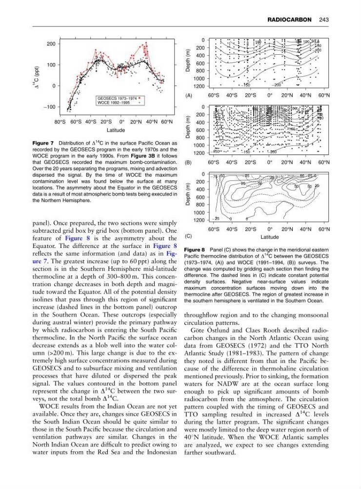
panel). Once prepared, the two sections were simply
subtracted grid box by grid box (bottom panel). One
feature of Figure 8 is the asymmetry about the
Equator. The difference at the surface in Figure 8
reflects the same information (and data) as in Figure 7. The greatest increase (up to 60 ppt) along the
section is in the Southern Hemisphere mid-latitude
thermocline at a depth of 300–800 m. This concentration change decreases in both depth and magnitude toward the Equator. All of the potential density
isolines that pass through this region of significant
increase (dashed lines in the bottom panel) outcrop
in the Southern Ocean. These outcrops (especially
during austral winter) provide the primary pathway
by which radiocarbon is entering the South Pacific
thermocline. In the North Pacific the surface ocean
decrease extends as a blob well into the water column (>200 m). This large change is due to the extremely high surface concentrations measured during
GEOSECS and to subsurface mixing and ventilation
processes that have diluted or dispersed the peak
signal. The values contoured in the bottom panel
represent the change in D
14 C between the two surveys, not the total bomb D
14
C.
WOCE results from the Indian Ocean are not yet
available. Once they are, changes since GEOSECS in
the South Indian Ocean should be quite similar to
those in the South Pacific because the circulation and
ventilation pathways are similar. Changes in the
North Indian Ocean are difficult to predict owing to
water inputs from the Red Sea and the Indonesian
throughflow region and to the changing monsoonal
circulation patterns.
Go ¨ te O ¨ stlund and Claes Rooth described radiocarbon changes in the North Atlantic Ocean using
data from GEOSECS (1972) and the TTO North
Atlantic Study (1981–1983). The pattern of change
they noted is different from that in the Pacific because of the difference in thermohaline circulation
mentioned previously. Prior to sinking, the formation
waters for NADW are at the ocean surface long
enough to pick up significant amounts of bomb
radiocarbon from the atmosphere. The circulation
pattern coupled with the timing of GEOSECS and
TTO sampling resulted in increased D
14 C levels
during the latter program. The significant changes
were mostly limited to the deep water region north of
401N latitude. When the WOCE Atlantic samples
are analyzed, we expect to see changes extending
farther southward.
GEOSECS 1973 1974
−
WOCE 1992 1995
−
_ 100
0
100
200
80°S 60°S 40°S 20°S
20°N 40°N 60°N
Latitude
0°
Δ
14
C (ppt)
Figure 7 Distribution of D
14
C in the surface Pacific Ocean as
recorded by the GEOSECS program in the early 1970s and the
WOCE program in the early 1990s. From Figure 3B it follows
that GEOSECS recorded the maximum bomb-contamination.
Over the 20 years separating the programs, mixing and advection
dispersed the signal. By the time of WOCE the maximum
contamination level was found below the surface at many
locations. The asymmetry about the Equator in the GEOSECS
data is a result of most atmospheric bomb tests being executed in
the Northern Hemisphere.
_ 200
_ 150
_ 100
_ 50
0
50
100
100
150
•
•
• •
•
•
•
•
•
•
• •
•
•
•
•
•
•
•
•
•
•
•
•
•
•
•
•
•
•
• • •
•
•
•
•
• •
• •
•
•
•
•
•
•
•
•
•
• •
•
•
•
•
•
•
•
•
•
•
•
•
•
•
•
•
•
•
•
•
•
•
•
•
•
•
•
• •
• •
•
•
•
•
•
•
•
•
•
•
•
•
•
•
•
•
•
•
• •
•
•
•
•
•
•
•
• •
• •
•
•
•
•
•
•
•
•
•
•
•
•
•
• •
• •
• •
•
•
•
•
•
•
•
• • •
•
•
•
•
•
•
•
• • •
• •
• •
•
•
•
•
•
•
•
• • • •
•
•
•
•
•
•
• •
•
•
•
•
•
•
•
•
•
•
•
•
•
•
•
• • •
•
• • •
•
• •
•
•
•
•
•
•
•
•
•
•
• • •
•
•
•
•
•
•
•
•
• •
•
•
•
•
•
•
•
• • •
•
•
•
•
•
•
•
•
•
•
•
•
•
•
•
•
•
•
•
•
•
•
•
•
•
•
•
•
• •
•
•
•
•
•
•
•
•
•
•
•
• •
•
•
•
•
• •
•
•
•
•
•
_ 200
_ 150
_ 150
_ 100
_ 100
_ 50
0
50
100
100
• • • •
•
•
•
•
•
•
•
•
• • • •
• •
•
•
•
•
•
• • • • • •
• • •
•
•
•
•
•
•
•
•
•
•
•
•
•
• • • •
•
•
•
•
•
• • • •
• •
•
•
•
•
•
•
•
•
•
•
• • •
•
• •
•
•
•
•
•
•
•
•
•
• • • •
•
•
•
•
•
•
• • •
• • •
•
•
•
•
•
• • •
•
•
•
•
•
•
•
•
•
•
•
•
•
•
•
•
•
•
•
•
•
•
•
•
•
• •
• • • • •
•
•
•
•
•
•
•
•
•
• • •
•
•
•
•
•
•
•
•
•
•
•
•
•
• •
• •
•
•
•
•
•
•
•
•
•
•
•
•
•
•
•
•
•
•
•
•
•
•
•
•
•
•
•
•
•
•
•
•
•
•
•
•
•
•
•
•
•
•
•
•
•
•
•
•
•
•
•
•
•
• • • •
•
•
•
•
•
•
•
•
• •
•
•
•
•
•
•
•
•
•
• • • •
• •
•
•
•
•
•
•
• • •
•
• •
•
•
•
•
•
•
•
•
•
•
•
• •
•
•
• • •
•
•
•
•
• • • • • • • • • • • • • •
•
•
•
•
•
•
•
•
• • • • • •
•
• •
•
•
•
•
•
•
• • • • • • • • • • • •
•
•
•
•
•
•
•
• • • •
• • • • • • •
•
•
•
•
•
• •
•
•
• • • • • • • • • •
• •
•
•
•
•
•
• •
•
• • • • • •
• •
•
•
•
•
•
•
•
•
• • • •
•
•
• •
• •
•
•
•
• •
• • • •
•
•
• •
•
•
•
• • • • • • • •
• • •
•
•
•
• •
•
• • • • • • •
• •
• • •
•
•
•
• • • • •
• • • • • • •
•
•
• • • • • • • • • • •
•
•
•
•
• • • • • •
• •
• •
•
•
•
•
•
•
• • •
• • •
•
•
•
•
• • • • • • • •
•
•
•
•
•
•
• •
• • • • • •
• •
• •
•
•
•
• • • • • • • • • •
•
•
•
•
•
••
• • • • •
• •
•
•
•
•
•
•
•
•
• • • •
• • •
•
•
•
•
•
• •
•
•
• • •
•
• •
•
•
•
•
•
•
•
• • • • •
• • • • • •
•
•
•
•
•
•
•
•
• •
•
• • •
•
•
•
•
• • • •
• •
• •
•
•
•
•
•
•
•
•
• • • • •
• •
• • • •
• •
•
•
• •
• •
• •
• • • •
•
•
•
•
•
•
•
•
•
•
•
•
•
•
•
• •
•
•
•
•
•
•
•
•
•
•
• • •
•
•
• •
•
•
• •
•
• • • • •
• •
•
•
•
•
•
•
•
• •
• •
•
• • • •
•
• •
•
• •
•
• • • • • •
• •
•
• •
•
•
• •
•
• • •
•
•
•
•
•
•
•
•
•
• •
• • • • • • • •
•
• •
•
• •
•
•
•
• • •
• • • • • •
• • •
•
• •
• •
• •
• •
•
• • • •
•
•
•
•
•
•
•
•
• • • •
•
•
•
•
•
•
•
•
• • • • •
•
• •
• • •
•
•
•
• •
•
• • • • •
• •
Latitude
Depth (m)
60°S 40°S
20°S
0°
20°N 40°N 60°N
1200
600
200
_ 75
_ 50
_ 50
_ 25
_ 25
_ 25
0
0
0
25
25
25
50
50
50
60°S 40°S
20°S
0°
20°N 40°N 60°N
60°S 40°S
20°S
0°
20°N 40°N 60°N
Depth (m)
1200
600
200
Depth (m)
1200
600
200
(A)
(B)
(C)
1000
800
400
0
1000
800
400
0
1000
800
400
0
Figure 8 Panel (C) shows the change in the meridional eastern
Pacific thermocline distribution of D
14 C between the GEOSECS
(1973–1974, (A)) and WOCE (1991–1994, (B)) surveys. The
change was computed by gridding each section then finding the
difference. The dashed lines in (C) indicate constant potential
density surfaces. Negative near-surface values indicate
maximum concentration surfaces moving down into the
thermocline after GEOSECS. The region of greatest increase in
the southern hemisphere is ventilated in the Southern Ocean.
RADIOCARBON 243
subtracted grid box by grid box (bottom panel). One
feature of Figure 8 is the asymmetry about the
Equator. The difference at the surface in Figure 8
reflects the same information (and data) as in Figure 7. The greatest increase (up to 60 ppt) along the
section is in the Southern Hemisphere mid-latitude
thermocline at a depth of 300–800 m. This concentration change decreases in both depth and magnitude toward the Equator. All of the potential density
isolines that pass through this region of significant
increase (dashed lines in the bottom panel) outcrop
in the Southern Ocean. These outcrops (especially
during austral winter) provide the primary pathway
by which radiocarbon is entering the South Pacific
thermocline. In the North Pacific the surface ocean
decrease extends as a blob well into the water column (>200 m). This large change is due to the extremely high surface concentrations measured during
GEOSECS and to subsurface mixing and ventilation
processes that have diluted or dispersed the peak
signal. The values contoured in the bottom panel
represent the change in D
14 C between the two surveys, not the total bomb D
14
C.
WOCE results from the Indian Ocean are not yet
available. Once they are, changes since GEOSECS in
the South Indian Ocean should be quite similar to
those in the South Pacific because the circulation and
ventilation pathways are similar. Changes in the
North Indian Ocean are difficult to predict owing to
water inputs from the Red Sea and the Indonesian
throughflow region and to the changing monsoonal
circulation patterns.
Go ¨ te O ¨ stlund and Claes Rooth described radiocarbon changes in the North Atlantic Ocean using
data from GEOSECS (1972) and the TTO North
Atlantic Study (1981–1983). The pattern of change
they noted is different from that in the Pacific because of the difference in thermohaline circulation
mentioned previously. Prior to sinking, the formation
waters for NADW are at the ocean surface long
enough to pick up significant amounts of bomb
radiocarbon from the atmosphere. The circulation
pattern coupled with the timing of GEOSECS and
TTO sampling resulted in increased D
14 C levels
during the latter program. The significant changes
were mostly limited to the deep water region north of
401N latitude. When the WOCE Atlantic samples
are analyzed, we expect to see changes extending
farther southward.
GEOSECS 1973 1974
−
WOCE 1992 1995
−
_ 100
0
100
200
80°S 60°S 40°S 20°S
20°N 40°N 60°N
Latitude
0°
Δ
14
C (ppt)
Figure 7 Distribution of D
14
C in the surface Pacific Ocean as
recorded by the GEOSECS program in the early 1970s and the
WOCE program in the early 1990s. From Figure 3B it follows
that GEOSECS recorded the maximum bomb-contamination.
Over the 20 years separating the programs, mixing and advection
dispersed the signal. By the time of WOCE the maximum
contamination level was found below the surface at many
locations. The asymmetry about the Equator in the GEOSECS
data is a result of most atmospheric bomb tests being executed in
the Northern Hemisphere.
_ 200
_ 150
_ 100
_ 50
0
50
100
100
150
•
•
• •
•
•
•
•
•
•
• •
•
•
•
•
•
•
•
•
•
•
•
•
•
•
•
•
•
•
• • •
•
•
•
•
• •
• •
•
•
•
•
•
•
•
•
•
• •
•
•
•
•
•
•
•
•
•
•
•
•
•
•
•
•
•
•
•
•
•
•
•
•
•
•
•
• •
• •
•
•
•
•
•
•
•
•
•
•
•
•
•
•
•
•
•
•
• •
•
•
•
•
•
•
•
• •
• •
•
•
•
•
•
•
•
•
•
•
•
•
•
• •
• •
• •
•
•
•
•
•
•
•
• • •
•
•
•
•
•
•
•
• • •
• •
• •
•
•
•
•
•
•
•
• • • •
•
•
•
•
•
•
• •
•
•
•
•
•
•
•
•
•
•
•
•
•
•
•
• • •
•
• • •
•
• •
•
•
•
•
•
•
•
•
•
•
• • •
•
•
•
•
•
•
•
•
• •
•
•
•
•
•
•
•
• • •
•
•
•
•
•
•
•
•
•
•
•
•
•
•
•
•
•
•
•
•
•
•
•
•
•
•
•
•
• •
•
•
•
•
•
•
•
•
•
•
•
• •
•
•
•
•
• •
•
•
•
•
•
_ 200
_ 150
_ 150
_ 100
_ 100
_ 50
0
50
100
100
• • • •
•
•
•
•
•
•
•
•
• • • •
• •
•
•
•
•
•
• • • • • •
• • •
•
•
•
•
•
•
•
•
•
•
•
•
•
• • • •
•
•
•
•
•
• • • •
• •
•
•
•
•
•
•
•
•
•
•
• • •
•
• •
•
•
•
•
•
•
•
•
•
• • • •
•
•
•
•
•
•
• • •
• • •
•
•
•
•
•
• • •
•
•
•
•
•
•
•
•
•
•
•
•
•
•
•
•
•
•
•
•
•
•
•
•
•
• •
• • • • •
•
•
•
•
•
•
•
•
•
• • •
•
•
•
•
•
•
•
•
•
•
•
•
•
• •
• •
•
•
•
•
•
•
•
•
•
•
•
•
•
•
•
•
•
•
•
•
•
•
•
•
•
•
•
•
•
•
•
•
•
•
•
•
•
•
•
•
•
•
•
•
•
•
•
•
•
•
•
•
•
• • • •
•
•
•
•
•
•
•
•
• •
•
•
•
•
•
•
•
•
•
• • • •
• •
•
•
•
•
•
•
• • •
•
• •
•
•
•
•
•
•
•
•
•
•
•
• •
•
•
• • •
•
•
•
•
• • • • • • • • • • • • • •
•
•
•
•
•
•
•
•
• • • • • •
•
• •
•
•
•
•
•
•
• • • • • • • • • • • •
•
•
•
•
•
•
•
• • • •
• • • • • • •
•
•
•
•
•
• •
•
•
• • • • • • • • • •
• •
•
•
•
•
•
• •
•
• • • • • •
• •
•
•
•
•
•
•
•
•
• • • •
•
•
• •
• •
•
•
•
• •
• • • •
•
•
• •
•
•
•
• • • • • • • •
• • •
•
•
•
• •
•
• • • • • • •
• •
• • •
•
•
•
• • • • •
• • • • • • •
•
•
• • • • • • • • • • •
•
•
•
•
• • • • • •
• •
• •
•
•
•
•
•
•
• • •
• • •
•
•
•
•
• • • • • • • •
•
•
•
•
•
•
• •
• • • • • •
• •
• •
•
•
•
• • • • • • • • • •
•
•
•
•
•
••
• • • • •
• •
•
•
•
•
•
•
•
•
• • • •
• • •
•
•
•
•
•
• •
•
•
• • •
•
• •
•
•
•
•
•
•
•
• • • • •
• • • • • •
•
•
•
•
•
•
•
•
• •
•
• • •
•
•
•
•
• • • •
• •
• •
•
•
•
•
•
•
•
•
• • • • •
• •
• • • •
• •
•
•
• •
• •
• •
• • • •
•
•
•
•
•
•
•
•
•
•
•
•
•
•
•
• •
•
•
•
•
•
•
•
•
•
•
• • •
•
•
• •
•
•
• •
•
• • • • •
• •
•
•
•
•
•
•
•
• •
• •
•
• • • •
•
• •
•
• •
•
• • • • • •
• •
•
• •
•
•
• •
•
• • •
•
•
•
•
•
•
•
•
•
• •
• • • • • • • •
•
• •
•
• •
•
•
•
• • •
• • • • • •
• • •
•
• •
• •
• •
• •
•
• • • •
•
•
•
•
•
•
•
•
• • • •
•
•
•
•
•
•
•
•
• • • • •
•
• •
• • •
•
•
•
• •
•
• • • • •
• •
Latitude
Depth (m)
60°S 40°S
20°S
0°
20°N 40°N 60°N
1200
600
200
_ 75
_ 50
_ 50
_ 25
_ 25
_ 25
0
0
0
25
25
25
50
50
50
60°S 40°S
20°S
0°
20°N 40°N 60°N
60°S 40°S
20°S
0°
20°N 40°N 60°N
Depth (m)
1200
600
200
Depth (m)
1200
600
200
(A)
(B)
(C)
1000
800
400
0
1000
800
400
0
1000
800
400
0
Figure 8 Panel (C) shows the change in the meridional eastern
Pacific thermocline distribution of D
14 C between the GEOSECS
(1973–1974, (A)) and WOCE (1991–1994, (B)) surveys. The
change was computed by gridding each section then finding the
difference. The dashed lines in (C) indicate constant potential
density surfaces. Negative near-surface values indicate
maximum concentration surfaces moving down into the
thermocline after GEOSECS. The region of greatest increase in
the southern hemisphere is ventilated in the Southern Ocean.
RADIOCARBON 243