

observations d i 7s i :
Fðp
à ; ˜
pÞ ¼ ? þ
m i À d i
s i
! 2
þ ?
½11
A large value of F indicates that the simulated tracer
concentrations differ much from the observations.
Bringing the model close to the data, therefore, is
equivalent to minimizing F, subject to satisfying the
model equations (tracer budget equations) E j ¼ 0
exactly.
Details on the Lagrange multiplier method used
for the constrained minimization of F can be found
in textbooks and the literature on data assimilation
or constrained data fitting. Overall, this method
allows calculating the direction in parameter space
ÀrF p à of steepest decrease of F (the negative gradient of F with respect to p
à ), which can then be used
by a descent algorithm to arrive at a new, modified
vector of independent parameters p
à . It is guaranteed
that new simulations using the modified p
à will lead
to more realistic tracer simulations and a smaller
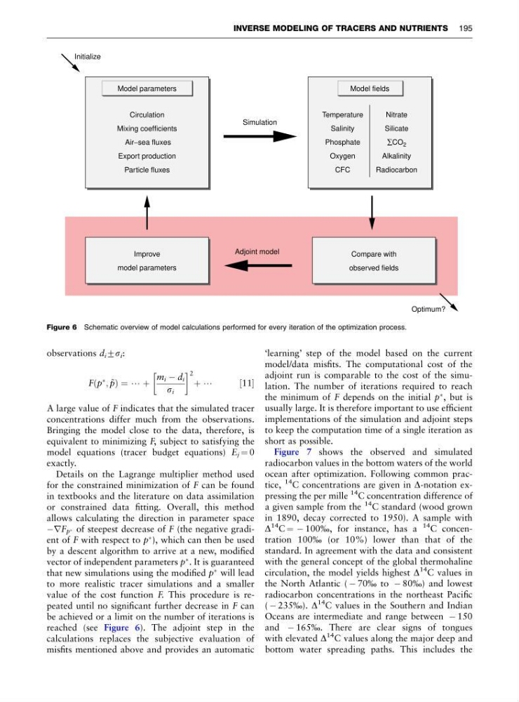
value of the cost function F. This procedure is repeated until no significant further decrease in F can
be achieved or a limit on the number of iterations is
reached (see Figure 6). The adjoint step in the
calculations replaces the subjective evaluation of
misfits mentioned above and provides an automatic
‘learning’ step of the model based on the current
model/data misfits. The computational cost of the
adjoint run is comparable to the cost of the simulation. The number of iterations required to reach
the minimum of F depends on the initial p
à , but is
usually large. It is therefore important to use efficient
implementations of the simulation and adjoint steps
to keep the computation time of a single iteration as
short as possible.
Figure 7 shows the observed and simulated
radiocarbon values in the bottom waters of the world
ocean after optimization. Following common practice,
14 C concentrations are given in D-notation expressing the per mille
14 C concentration difference of
a given sample from the
14 C standard (wood grown
in 1890, decay corrected to 1950). A sample with
D
14
C ¼ À 100%, for instance, has a
14
C concentration 100% (or 10%) lower than that of the
standard. In agreement with the data and consistent
with the general concept of the global thermohaline
circulation, the model yields highest D
14 C values in
the North Atlantic ( À 70% to À 80%) and lowest
radiocarbon concentrations in the northeast Pacific
( À 235%). D
14
C values in the Southern and Indian
Oceans are intermediate and range between À 150
and À 165%. There are clear signs of tongues
with elevated D
14 C values along the major deep and
bottom water spreading paths. This includes the
Circulation
Mixing coefficients
Air−sea fluxes
Export production
Particle fluxes
Simulation
Adjoint model
Initialize
Optimum?
Temperature
Salinity
Phosphate
Oxygen
CFC
Nitrate
Silicate
∑CO 2
Alkalinity
Radiocarbon
Improve
model parameters
Compare with
observed fields
Model fields
Model parameters
Figure 6 Schematic overview of model calculations performed for every iteration of the optimization process.
INVERSE MODELING OF TRACERS AND NUTRIENTS 195
Fðp
à ; ˜
pÞ ¼ ? þ
m i À d i
s i
! 2
þ ?
½11
A large value of F indicates that the simulated tracer
concentrations differ much from the observations.
Bringing the model close to the data, therefore, is
equivalent to minimizing F, subject to satisfying the
model equations (tracer budget equations) E j ¼ 0
exactly.
Details on the Lagrange multiplier method used
for the constrained minimization of F can be found
in textbooks and the literature on data assimilation
or constrained data fitting. Overall, this method
allows calculating the direction in parameter space
ÀrF p à of steepest decrease of F (the negative gradient of F with respect to p
à ), which can then be used
by a descent algorithm to arrive at a new, modified
vector of independent parameters p
à . It is guaranteed
that new simulations using the modified p
à will lead
to more realistic tracer simulations and a smaller
value of the cost function F. This procedure is repeated until no significant further decrease in F can
be achieved or a limit on the number of iterations is
reached (see Figure 6). The adjoint step in the
calculations replaces the subjective evaluation of
misfits mentioned above and provides an automatic
‘learning’ step of the model based on the current
model/data misfits. The computational cost of the
adjoint run is comparable to the cost of the simulation. The number of iterations required to reach
the minimum of F depends on the initial p
à , but is
usually large. It is therefore important to use efficient
implementations of the simulation and adjoint steps
to keep the computation time of a single iteration as
short as possible.
Figure 7 shows the observed and simulated
radiocarbon values in the bottom waters of the world
ocean after optimization. Following common practice,
14 C concentrations are given in D-notation expressing the per mille
14 C concentration difference of
a given sample from the
14 C standard (wood grown
in 1890, decay corrected to 1950). A sample with
D
14
C ¼ À 100%, for instance, has a
14
C concentration 100% (or 10%) lower than that of the
standard. In agreement with the data and consistent
with the general concept of the global thermohaline
circulation, the model yields highest D
14 C values in
the North Atlantic ( À 70% to À 80%) and lowest
radiocarbon concentrations in the northeast Pacific
( À 235%). D
14
C values in the Southern and Indian
Oceans are intermediate and range between À 150
and À 165%. There are clear signs of tongues
with elevated D
14 C values along the major deep and
bottom water spreading paths. This includes the
Circulation
Mixing coefficients
Air−sea fluxes
Export production
Particle fluxes
Simulation
Adjoint model
Initialize
Optimum?
Temperature
Salinity
Phosphate
Oxygen
CFC
Nitrate
Silicate
∑CO 2
Alkalinity
Radiocarbon
Improve
model parameters
Compare with
observed fields
Model fields
Model parameters
Figure 6 Schematic overview of model calculations performed for every iteration of the optimization process.
INVERSE MODELING OF TRACERS AND NUTRIENTS 195