

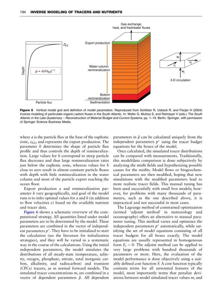
where a is the particle flux at the base of the euphotic
zone, z EZ , and represents the export production. The
parameter b determines the shape of particle flux
profile and thus controls the depth of remineralization. Large values for b correspond to steep particle
flux decreases and thus large remineralization rates
just below the euphotic zone, whereas values for b
close to zero result in almost constant particle fluxes
with depth with little remineralization in the water
column and most of the particle export reaching the
ocean floor.
Export production a and remineralization parameter b vary geographically, and goal of the model
runs is to infer optimal values for a and b (in addition
to flow velocities v) based on the available nutrient
and tracer data.
Figure 6 shows a schematic overview of the computational strategy. All quantities listed under model
parameters are to be determined by the model. These
parameters are combined in the vector of independent parameters p
à . They have to be initialized to start
the calculation (see the literature for initialization
strategies), and they will be varied in a systematic
way in the course of the calculations. Using the initial
independent parameters, the model simulates the
distributions of all steady-state (temperature, salinity, oxygen, phosphate, nitrate, total inorganic carbon, alkalinity, and radiocarbon) and transient
(CFCs) tracers, as in normal forward models. The
simulated tracer concentrations m i are combined in a
vector of dependent parameters ˜
p. All dependent
parameters in ˜
p can be calculated uniquely from the
independent parameters p
à using the tracer budget
equations for the boxes of the model.
Once calculated, the simulated tracer distributions
can be compared with measurements. Traditionally,
this model/data comparison is done subjectively by
analyzing the misfit fields and hypothesizing possible
causes for the misfits. Model flows or biogeochemical parameters are then modified, hoping that new
simulations with the modified parameters lead to
more realistic tracer fields. This manual tuning has
been used successfully with small box models; however, for problems with many thousands of parameters, such as the one described above, it is
impractical and not successful in most cases.
The Lagrange method of constrained optimization
(termed ‘adjoint method’ in meteorology and
oceanography) offers an alternative to manual parameter tuning. This method varies and optimizes the
independent parameters p
à automatically, while satisfying the set of model equations consisting of all
tracer budgets for all boxes exactly. The model
equations are usually represented in homogeneous
form E j ¼ 0. The adjoint method can be applied to
very large problems with hundred thousands of
parameters or more. Here, the evaluation of the
model performance is done objectively using a suitably defined cost function F. A cost function typically
contains terms for all unwanted features of the
model, most importantly terms that penalize deviations between model simulated tracer values m i and
Gas exchange,
heat, and freshwater fluxes
Export production
Z EZ
Depth
Water-column
remineralization
Bottom
remineralization
Sedimentation
w i
w j
u j
v i
3-D circulation
Particle flux
Figure 5 Vertical model grid and definition of model parameters. Reproduced from Schlitzer R, Usbeck R, and Fiscjer H (2004)
Inverse modeling of particulate organic carbon fluxes in the South Atlantic. In: Wefer G, Mulitza S, and Ratmeyer V (eds.) The South
Atlantic in the Late Quaternary – Reconstruction of Material Budget and Current Systems, pp. 1–19. Berlin: Springer, with permission
of Springer Science Business Media.
194 INVERSE MODELING OF TRACERS AND NUTRIENTS
zone, z EZ , and represents the export production. The
parameter b determines the shape of particle flux
profile and thus controls the depth of remineralization. Large values for b correspond to steep particle
flux decreases and thus large remineralization rates
just below the euphotic zone, whereas values for b
close to zero result in almost constant particle fluxes
with depth with little remineralization in the water
column and most of the particle export reaching the
ocean floor.
Export production a and remineralization parameter b vary geographically, and goal of the model
runs is to infer optimal values for a and b (in addition
to flow velocities v) based on the available nutrient
and tracer data.
Figure 6 shows a schematic overview of the computational strategy. All quantities listed under model
parameters are to be determined by the model. These
parameters are combined in the vector of independent parameters p
à . They have to be initialized to start
the calculation (see the literature for initialization
strategies), and they will be varied in a systematic
way in the course of the calculations. Using the initial
independent parameters, the model simulates the
distributions of all steady-state (temperature, salinity, oxygen, phosphate, nitrate, total inorganic carbon, alkalinity, and radiocarbon) and transient
(CFCs) tracers, as in normal forward models. The
simulated tracer concentrations m i are combined in a
vector of dependent parameters ˜
p. All dependent
parameters in ˜
p can be calculated uniquely from the
independent parameters p
à using the tracer budget
equations for the boxes of the model.
Once calculated, the simulated tracer distributions
can be compared with measurements. Traditionally,
this model/data comparison is done subjectively by
analyzing the misfit fields and hypothesizing possible
causes for the misfits. Model flows or biogeochemical parameters are then modified, hoping that new
simulations with the modified parameters lead to
more realistic tracer fields. This manual tuning has
been used successfully with small box models; however, for problems with many thousands of parameters, such as the one described above, it is
impractical and not successful in most cases.
The Lagrange method of constrained optimization
(termed ‘adjoint method’ in meteorology and
oceanography) offers an alternative to manual parameter tuning. This method varies and optimizes the
independent parameters p
à automatically, while satisfying the set of model equations consisting of all
tracer budgets for all boxes exactly. The model
equations are usually represented in homogeneous
form E j ¼ 0. The adjoint method can be applied to
very large problems with hundred thousands of
parameters or more. Here, the evaluation of the
model performance is done objectively using a suitably defined cost function F. A cost function typically
contains terms for all unwanted features of the
model, most importantly terms that penalize deviations between model simulated tracer values m i and
Gas exchange,
heat, and freshwater fluxes
Export production
Z EZ
Depth
Water-column
remineralization
Bottom
remineralization
Sedimentation
w i
w j
u j
v i
3-D circulation
Particle flux
Figure 5 Vertical model grid and definition of model parameters. Reproduced from Schlitzer R, Usbeck R, and Fiscjer H (2004)
Inverse modeling of particulate organic carbon fluxes in the South Atlantic. In: Wefer G, Mulitza S, and Ratmeyer V (eds.) The South
Atlantic in the Late Quaternary – Reconstruction of Material Budget and Current Systems, pp. 1–19. Berlin: Springer, with permission
of Springer Science Business Media.
194 INVERSE MODELING OF TRACERS AND NUTRIENTS