

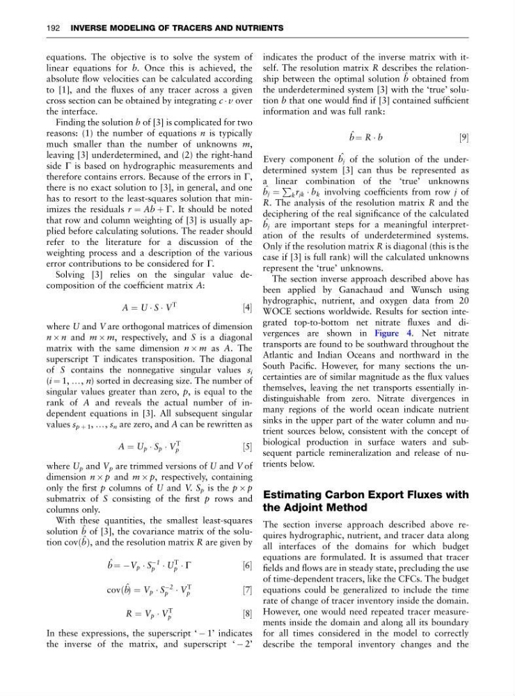
equations. The objective is to solve the system of
linear equations for b. Once this is achieved, the
absolute flow velocities can be calculated according
to [1], and the fluxes of any tracer across a given
cross section can be obtained by integrating c Á v over
the interface.
Finding the solution b of [3] is complicated for two
reasons: (1) the number of equations n is typically
much smaller than the number of unknowns m,
leaving [3] underdetermined, and (2) the right-hand
side G is based on hydrographic measurements and
therefore contains errors. Because of the errors in G,
there is no exact solution to [3], in general, and one
has to resort to the least-squares solution that minimizes the residuals r ¼ Ab þ G. It should be noted
that row and column weighting of [3] is usually applied before calculating solutions. The reader should
refer to the literature for a discussion of the
weighting process and a description of the various
error contributions to be considered for G.
Solving [3] relies on the singular value decomposition of the coefficient matrix A:
A ¼ U Á S Á V
T
½4
where U and V are orthogonal matrices of dimension
n  n and m  m, respectively, and S is a diagonal
matrix with the same dimension n  m as A. The
superscript T indicates transposition. The diagonal
of S contains the nonnegative singular values s i
(i ¼ 1, y, n) sorted in decreasing size. The number of
singular values greater than zero, p, is equal to the
rank of A and reveals the actual number of independent equations in [3]. All subsequent singular
values s p þ 1 , y, s n are zero, and A can be rewritten as
A ¼ U p Á S p Á V
T
p
½5
where U p and V p are trimmed versions of U and V of
dimension n  p and m  p, respectively, containing
only the first p columns of U and V. S p is the p  p
submatrix of S consisting of the first p rows and
columns only.
With these quantities, the smallest least-squares
solution b ˆ of [3], the covariance matrix of the solution covðb ˆ Þ, and the resolution matrix R are given by
b ˆ ¼ ÀV p Á S
À1
p Á U
T
p Á G
½6
covðb ˆ Þ ¼ V p Á S
À2
p Á V
T
p
½7
R ¼ V p Á V
T
p
½8
In these expressions, the superscript ‘ À 1’ indicates
the inverse of the matrix, and superscript ‘ À 2’
indicates the product of the inverse matrix with itself. The resolution matrix R describes the relationship between the optimal solution b ˆ obtained from
the underdetermined system [3] with the ‘true’ solution b that one would find if [3] contained sufficient
information and was full rank:
b ˆ ¼ R Á b
½9
Every component b ˆ j of the solution of the underdetermined system [3] can thus be represented as
a linear combination of the ‘true’ unknowns
b ˆ j ¼
P
k r jk Á b k involving coefficients from row j of
R. The analysis of the resolution matrix R and the
deciphering of the real significance of the calculated
b ˆ j are important steps for a meaningful interpretation of the results of underdetermined systems.
Only if the resolution matrix R is diagonal (this is the
case if [3] is full rank) will the calculated unknowns
represent the ‘true’ unknowns.
The section inverse approach described above has
been applied by Ganachaud and Wunsch using
hydrographic, nutrient, and oxygen data from 20
WOCE sections worldwide. Results for section integrated top-to-bottom net nitrate fluxes and divergences are shown in Figure 4. Net nitrate
transports are found to be southward throughout the
Atlantic and Indian Oceans and northward in the
South Pacific. However, for many sections the uncertainties are of similar magnitude as the flux values
themselves, leaving the net transports essentially indistinguishable from zero. Nitrate divergences in
many regions of the world ocean indicate nutrient
sinks in the upper part of the water column and nutrient sources below, consistent with the concept of
biological production in surface waters and subsequent particle remineralization and release of nutrients below.
Estimating Carbon Export Fluxes with
the Adjoint Method
The section inverse approach described above requires hydrographic, nutrient, and tracer data along
all interfaces of the domains for which budget
equations are formulated. It is assumed that tracer
fields and flows are in steady state, precluding the use
of time-dependent tracers, like the CFCs. The budget
equations could be generalized to include the time
rate of change of tracer inventory inside the domain.
However, one would need repeated tracer measurements inside the domain and along all its boundary
for all times considered in the model to correctly
describe the temporal inventory changes and the
192 INVERSE MODELING OF TRACERS AND NUTRIENTS
linear equations for b. Once this is achieved, the
absolute flow velocities can be calculated according
to [1], and the fluxes of any tracer across a given
cross section can be obtained by integrating c Á v over
the interface.
Finding the solution b of [3] is complicated for two
reasons: (1) the number of equations n is typically
much smaller than the number of unknowns m,
leaving [3] underdetermined, and (2) the right-hand
side G is based on hydrographic measurements and
therefore contains errors. Because of the errors in G,
there is no exact solution to [3], in general, and one
has to resort to the least-squares solution that minimizes the residuals r ¼ Ab þ G. It should be noted
that row and column weighting of [3] is usually applied before calculating solutions. The reader should
refer to the literature for a discussion of the
weighting process and a description of the various
error contributions to be considered for G.
Solving [3] relies on the singular value decomposition of the coefficient matrix A:
A ¼ U Á S Á V
T
½4
where U and V are orthogonal matrices of dimension
n  n and m  m, respectively, and S is a diagonal
matrix with the same dimension n  m as A. The
superscript T indicates transposition. The diagonal
of S contains the nonnegative singular values s i
(i ¼ 1, y, n) sorted in decreasing size. The number of
singular values greater than zero, p, is equal to the
rank of A and reveals the actual number of independent equations in [3]. All subsequent singular
values s p þ 1 , y, s n are zero, and A can be rewritten as
A ¼ U p Á S p Á V
T
p
½5
where U p and V p are trimmed versions of U and V of
dimension n  p and m  p, respectively, containing
only the first p columns of U and V. S p is the p  p
submatrix of S consisting of the first p rows and
columns only.
With these quantities, the smallest least-squares
solution b ˆ of [3], the covariance matrix of the solution covðb ˆ Þ, and the resolution matrix R are given by
b ˆ ¼ ÀV p Á S
À1
p Á U
T
p Á G
½6
covðb ˆ Þ ¼ V p Á S
À2
p Á V
T
p
½7
R ¼ V p Á V
T
p
½8
In these expressions, the superscript ‘ À 1’ indicates
the inverse of the matrix, and superscript ‘ À 2’
indicates the product of the inverse matrix with itself. The resolution matrix R describes the relationship between the optimal solution b ˆ obtained from
the underdetermined system [3] with the ‘true’ solution b that one would find if [3] contained sufficient
information and was full rank:
b ˆ ¼ R Á b
½9
Every component b ˆ j of the solution of the underdetermined system [3] can thus be represented as
a linear combination of the ‘true’ unknowns
b ˆ j ¼
P
k r jk Á b k involving coefficients from row j of
R. The analysis of the resolution matrix R and the
deciphering of the real significance of the calculated
b ˆ j are important steps for a meaningful interpretation of the results of underdetermined systems.
Only if the resolution matrix R is diagonal (this is the
case if [3] is full rank) will the calculated unknowns
represent the ‘true’ unknowns.
The section inverse approach described above has
been applied by Ganachaud and Wunsch using
hydrographic, nutrient, and oxygen data from 20
WOCE sections worldwide. Results for section integrated top-to-bottom net nitrate fluxes and divergences are shown in Figure 4. Net nitrate
transports are found to be southward throughout the
Atlantic and Indian Oceans and northward in the
South Pacific. However, for many sections the uncertainties are of similar magnitude as the flux values
themselves, leaving the net transports essentially indistinguishable from zero. Nitrate divergences in
many regions of the world ocean indicate nutrient
sinks in the upper part of the water column and nutrient sources below, consistent with the concept of
biological production in surface waters and subsequent particle remineralization and release of nutrients below.
Estimating Carbon Export Fluxes with
the Adjoint Method
The section inverse approach described above requires hydrographic, nutrient, and tracer data along
all interfaces of the domains for which budget
equations are formulated. It is assumed that tracer
fields and flows are in steady state, precluding the use
of time-dependent tracers, like the CFCs. The budget
equations could be generalized to include the time
rate of change of tracer inventory inside the domain.
However, one would need repeated tracer measurements inside the domain and along all its boundary
for all times considered in the model to correctly
describe the temporal inventory changes and the
192 INVERSE MODELING OF TRACERS AND NUTRIENTS