

at a given station pair. The reference velocity b is left
unknown by the geostrophic calculation. Determining these unknowns was a major challenge in
physical oceanography for many decades. There is
one unknown reference velocity b i for every station
pair in the sections considered. Thus, for global
networks consisting of hundreds of sections, as in the
case of the WOCE survey, the number of unknown
velocities b i may amount to several thousands.
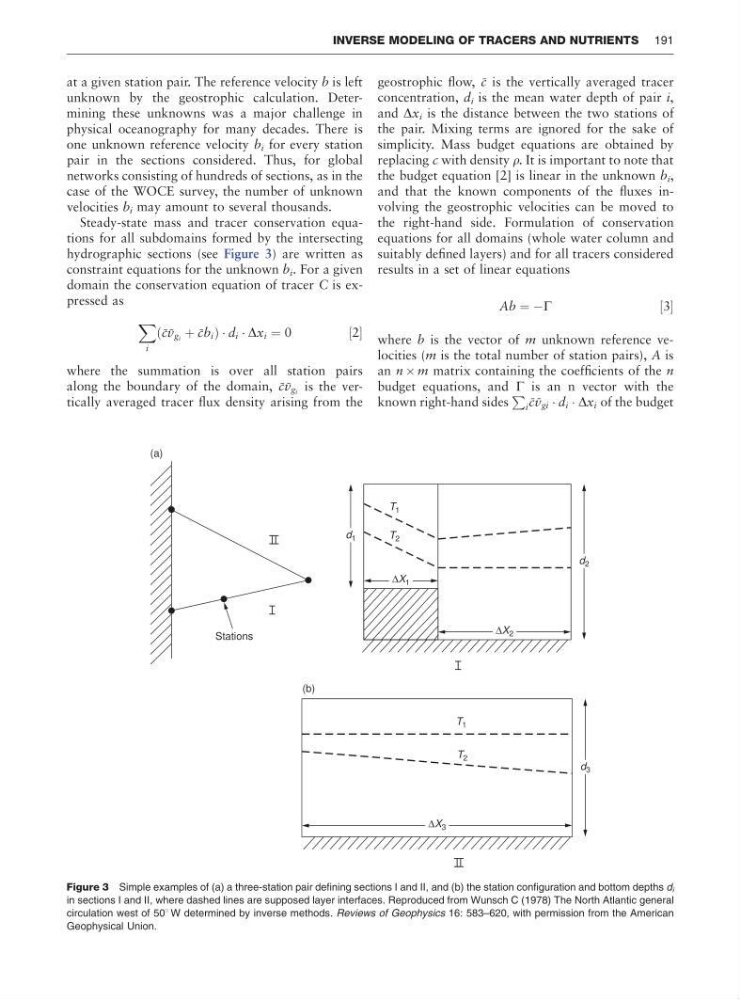
Steady-state mass and tracer conservation equations for all subdomains formed by the intersecting
hydrographic sections (see Figure 3) are written as
constraint equations for the unknown b i . For a given
domain the conservation equation of tracer C is expressed as
X
i
ð¯ c ¯
v g i þ ¯
cb i Þ Á d i Á Dx i ¼ 0
½2
where the summation is over all station pairs
along the boundary of the domain, ¯
c ¯
v gi is the vertically averaged tracer flux density arising from the
geostrophic flow, ¯
c is the vertically averaged tracer
concentration, d i is the mean water depth of pair i,
and Dx i is the distance between the two stations of
the pair. Mixing terms are ignored for the sake of
simplicity. Mass budget equations are obtained by
replacing c with density r. It is important to note that
the budget equation [2] is linear in the unknown b i ,
and that the known components of the fluxes involving the geostrophic velocities can be moved to
the right-hand side. Formulation of conservation
equations for all domains (whole water column and
suitably defined layers) and for all tracers considered
results in a set of linear equations
Ab ¼ ÀG
½3
where b is the vector of m unknown reference velocities (m is the total number of station pairs), A is
an n  m matrix containing the coefficients of the n
budget equations, and G is an n vector with the
known right-hand sides
P
i ¯
c ¯
v gi Á d i Á Dx i of the budget
Stations
(a)
(b)
T 1
T 1
T 2
T 2
d 1
d 2
d 3
ΔX 2
ΔX 1
ΔX 3
Figure 3 Simple examples of (a) a three-station pair defining sections I and II, and (b) the station configuration and bottom depths d i
in sections I and II, where dashed lines are supposed layer interfaces. Reproduced from Wunsch C (1978) The North Atlantic general
circulation west of 501 W determined by inverse methods. Reviews of Geophysics 16: 583–620, with permission from the American
Geophysical Union.
INVERSE MODELING OF TRACERS AND NUTRIENTS 191
unknown by the geostrophic calculation. Determining these unknowns was a major challenge in
physical oceanography for many decades. There is
one unknown reference velocity b i for every station
pair in the sections considered. Thus, for global
networks consisting of hundreds of sections, as in the
case of the WOCE survey, the number of unknown
velocities b i may amount to several thousands.
Steady-state mass and tracer conservation equations for all subdomains formed by the intersecting
hydrographic sections (see Figure 3) are written as
constraint equations for the unknown b i . For a given
domain the conservation equation of tracer C is expressed as
X
i
ð¯ c ¯
v g i þ ¯
cb i Þ Á d i Á Dx i ¼ 0
½2
where the summation is over all station pairs
along the boundary of the domain, ¯
c ¯
v gi is the vertically averaged tracer flux density arising from the
geostrophic flow, ¯
c is the vertically averaged tracer
concentration, d i is the mean water depth of pair i,
and Dx i is the distance between the two stations of
the pair. Mixing terms are ignored for the sake of
simplicity. Mass budget equations are obtained by
replacing c with density r. It is important to note that
the budget equation [2] is linear in the unknown b i ,
and that the known components of the fluxes involving the geostrophic velocities can be moved to
the right-hand side. Formulation of conservation
equations for all domains (whole water column and
suitably defined layers) and for all tracers considered
results in a set of linear equations
Ab ¼ ÀG
½3
where b is the vector of m unknown reference velocities (m is the total number of station pairs), A is
an n  m matrix containing the coefficients of the n
budget equations, and G is an n vector with the
known right-hand sides
P
i ¯
c ¯
v gi Á d i Á Dx i of the budget
Stations
(a)
(b)
T 1
T 1
T 2
T 2
d 1
d 2
d 3
ΔX 2
ΔX 1
ΔX 3
Figure 3 Simple examples of (a) a three-station pair defining sections I and II, and (b) the station configuration and bottom depths d i
in sections I and II, where dashed lines are supposed layer interfaces. Reproduced from Wunsch C (1978) The North Atlantic general
circulation west of 501 W determined by inverse methods. Reviews of Geophysics 16: 583–620, with permission from the American
Geophysical Union.
INVERSE MODELING OF TRACERS AND NUTRIENTS 191