

POPULATION CYCLES IN SMALL MAMMALS
317
June to October increase in weight only to 15-22 g and remain all
winter at these low weights. Chitty (1952) observed the same general
pattern for M . agrestis, and Kalela (1957) reported it for Clethrionomys
rufocanus. But while these seasonal variations have been clearly
described, few have tried to relate individual growth curves to density
changes.
Anderson (1970) emphasizes the distinction in growth and maturation
between spring- and fall-born animals, and refers to them as nearly
separate “generations”. There is little justification for such a clear-cut
1
$ -01I 1
1
1
1
1
1
1
t
1
1
,
0
10
20
30
4 0
50
BODY ‘WEIGHT - G
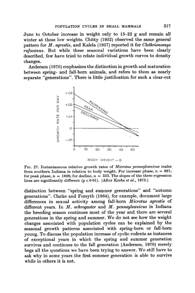
FIG. 27. Instantaneous relative growth rates of Microtus pennsylvanicus males
from southern Indiana in relation to body weight. For increase phase, n = 691;
for peak phase, n = 1898; for decline, n = 333. The slopes of the three regression
lines are significantly different (p < 0.01). (After Krebs et al., 1973.)
distinction between “spring and summer generations” and “autumn
generations”. Clarke and Forsyth (1964), for example, document large
differences in sexual activity among fall-born Microtus agrestis of
different years. In M . ochrogaster and M . pennsylvanicus in Indiana
the breeding season continues most of the year and there are several
generations in the spring and summer. We do not see how the weight
changes associated with population cycles can be explained by the
seasonal growth patterns associated with spring-born or fall-born
young. To discuss the population increase of cyclic rodents as instances
of exceptional years in which the spring and summer generation
survives and continues to the fall generation (Anderson, 1970) merely
begs all the questions we have been trying to answer. We still have to
ask why in some years the first summer generation is able to survive
while in others it is not.
317
June to October increase in weight only to 15-22 g and remain all
winter at these low weights. Chitty (1952) observed the same general
pattern for M . agrestis, and Kalela (1957) reported it for Clethrionomys
rufocanus. But while these seasonal variations have been clearly
described, few have tried to relate individual growth curves to density
changes.
Anderson (1970) emphasizes the distinction in growth and maturation
between spring- and fall-born animals, and refers to them as nearly
separate “generations”. There is little justification for such a clear-cut
1
$ -01I 1
1
1
1
1
1
1
t
1
1
,
0
10
20
30
4 0
50
BODY ‘WEIGHT - G
FIG. 27. Instantaneous relative growth rates of Microtus pennsylvanicus males
from southern Indiana in relation to body weight. For increase phase, n = 691;
for peak phase, n = 1898; for decline, n = 333. The slopes of the three regression
lines are significantly different (p < 0.01). (After Krebs et al., 1973.)
distinction between “spring and summer generations” and “autumn
generations”. Clarke and Forsyth (1964), for example, document large
differences in sexual activity among fall-born Microtus agrestis of
different years. In M . ochrogaster and M . pennsylvanicus in Indiana
the breeding season continues most of the year and there are several
generations in the spring and summer. We do not see how the weight
changes associated with population cycles can be explained by the
seasonal growth patterns associated with spring-born or fall-born
young. To discuss the population increase of cyclic rodents as instances
of exceptional years in which the spring and summer generation
survives and continues to the fall generation (Anderson, 1970) merely
begs all the questions we have been trying to answer. We still have to
ask why in some years the first summer generation is able to survive
while in others it is not.