

290
CHARLES J. D E B S AND JUDITH H. MYERS
20.0 -
15.0 -
E 10.0g 8 . 0 1
5 . 0 -
v)
0
>” 3 . 0 -
-
Y
0 2.00
Z
1.0 -
0.8 -
O
J
!
!
!
!
!
!
!
!
!
!
!
! I
A S O N D J
F M A M J
J
1963
1964
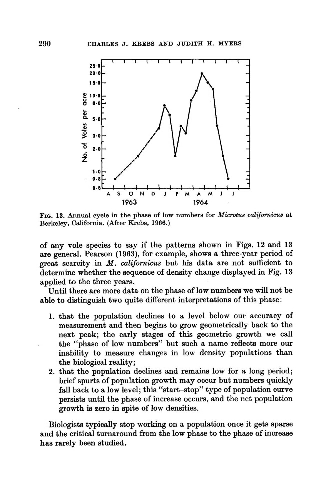
FIG. 13. Annual cycle in the phase of low numbers for Microtus cali,fornicua at
Berkeley, California. (After Krebs, 1966.)
of any vole species to say if the patterns shown in Figs. 12 and 13
are general. Pearson (1963), for example, shows a three-year period of
great scarcity in M . californicus but his data are not sufficient to
determine whether the sequence of density change displayed in Fig. 13
applied to the three years.
Until there are more data on the phase of low numbers we will not be
able to distinguish two quite different interpretations of this phase:
1. that the population declines to a level below our accuracy of
measurement and then begins to grow geometrically back to the
next peak; the early stages of this geometric growth we call
the “phase of low numbers” but such a name reflects more our
inability to measure changes in low density populations than
the biological reality;
2. that the population declines and remains low for a long period;
brief spurts of population growth may occur but numbers quickly
fall back to a low level; this “start-stop” type of population curve
persists until the phase of increase occurs, and the net population
growth is zero in spite of low densities.
.
Biologists typically stop working on a population once it gets sparse
and the critical turnaround from the low phase to the phase of increase
has rarely been studied.
CHARLES J. D E B S AND JUDITH H. MYERS
20.0 -
15.0 -
E 10.0g 8 . 0 1
5 . 0 -
v)
0
>” 3 . 0 -
-
Y
0 2.00
Z
1.0 -
0.8 -
O
J
!
!
!
!
!
!
!
!
!
!
!
! I
A S O N D J
F M A M J
J
1963
1964
FIG. 13. Annual cycle in the phase of low numbers for Microtus cali,fornicua at
Berkeley, California. (After Krebs, 1966.)
of any vole species to say if the patterns shown in Figs. 12 and 13
are general. Pearson (1963), for example, shows a three-year period of
great scarcity in M . californicus but his data are not sufficient to
determine whether the sequence of density change displayed in Fig. 13
applied to the three years.
Until there are more data on the phase of low numbers we will not be
able to distinguish two quite different interpretations of this phase:
1. that the population declines to a level below our accuracy of
measurement and then begins to grow geometrically back to the
next peak; the early stages of this geometric growth we call
the “phase of low numbers” but such a name reflects more our
inability to measure changes in low density populations than
the biological reality;
2. that the population declines and remains low for a long period;
brief spurts of population growth may occur but numbers quickly
fall back to a low level; this “start-stop” type of population curve
persists until the phase of increase occurs, and the net population
growth is zero in spite of low densities.
.
Biologists typically stop working on a population once it gets sparse
and the critical turnaround from the low phase to the phase of increase
has rarely been studied.