

250
WILLIAM STREIFER
This distribution corresponds to 26 animals with m c 0.7 mg and nine
animals with rn > 0-7 and nearly all of the distribution falls in the size
range of the animals Armstrong investigated.
5. Solution
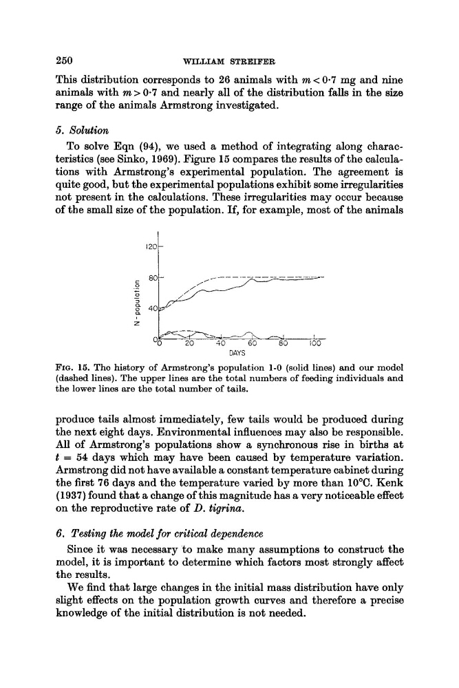
To solve Eqn (94), we used a method of integrating along characteristics (see Sinko, 1969). Figure 15 compares the results of the calculations with Armstrong’s experimental population. The agreement is
quite good, but the experimental populations exhibit some irregularities
not present in the calculations. These irregularities may occur because
of the small size of the population. If, for example, most of the animals
DAYS
FIG. 16. The history of Armstrong’s population 1-0 (solid lines) and our model
(dashed lines). The upper lines are the total numbers of feeding individuals and
the lower lines are the total number of tails.
produce tails almost immediately, few tails would be produced during
the next eight days. Environmental influences may also be responsible.
All of Armstrong’s populations show a synchronous rise in births at
t = 54 days which may have been caused by temperature variation.
Armstrong did not have available a constant temperature cabinet during
the first 76 days and the temperature varied by more than 10°C. Kenk
(1937) found that a change of this magnitude has a very noticeable effect
on the reproductive rate of D. tigrina.
6 . Testing the model for critical dependence
Since it was necessary to make many assumptions to construct the
model, it is important to determine which factors most strongly affect
the results.
We find that large changes in the initial mass distribution have only
slight effects on the population growth curves and therefore a precise
knowledge of the initial distribution is not needed.
WILLIAM STREIFER
This distribution corresponds to 26 animals with m c 0.7 mg and nine
animals with rn > 0-7 and nearly all of the distribution falls in the size
range of the animals Armstrong investigated.
5. Solution
To solve Eqn (94), we used a method of integrating along characteristics (see Sinko, 1969). Figure 15 compares the results of the calculations with Armstrong’s experimental population. The agreement is
quite good, but the experimental populations exhibit some irregularities
not present in the calculations. These irregularities may occur because
of the small size of the population. If, for example, most of the animals
DAYS
FIG. 16. The history of Armstrong’s population 1-0 (solid lines) and our model
(dashed lines). The upper lines are the total numbers of feeding individuals and
the lower lines are the total number of tails.
produce tails almost immediately, few tails would be produced during
the next eight days. Environmental influences may also be responsible.
All of Armstrong’s populations show a synchronous rise in births at
t = 54 days which may have been caused by temperature variation.
Armstrong did not have available a constant temperature cabinet during
the first 76 days and the temperature varied by more than 10°C. Kenk
(1937) found that a change of this magnitude has a very noticeable effect
on the reproductive rate of D. tigrina.
6 . Testing the model for critical dependence
Since it was necessary to make many assumptions to construct the
model, it is important to determine which factors most strongly affect
the results.
We find that large changes in the initial mass distribution have only
slight effects on the population growth curves and therefore a precise
knowledge of the initial distribution is not needed.