

REALISTIC MODELS IN POPULATION ECOLOGY
249
E
I - 0.75 t
I
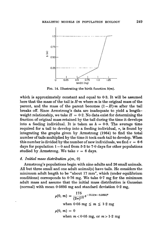
FIG. 14. Illustrating the birth function b(m).
which is approximately constant and equal to 0.3. It will be assumed
here that the mass of the tail is Hem where m is the original mass of the
parent, and the mass of the parent becomes (1 - H ) - m after the tail
breaks off. Since Armstrong’s data are inadequate to yield a lengthweight relationship, we take H = 0.2. No data exist for determining the
fraction of original mass retained by the tail during the time it develops
into a feeding individual. It is taken as h = 0.9. The average time
required for a tail to develop into a feeding individual, T , is found by
integrating the graphs given by Armstrong (1964) to find the total
number of tails multiplied by the time it took each tail to develop. When
this number is divided by the number of new individuals, we find T = 6.6
days for population 1 - 0 and from 5-3 to 7.0 days for other populations
studied by Armstrong. We take T = 6 days.
4. Initial mass distribution p(m, 0 )
Armstrong’s populations begin with nine adults and 26 small animals.
All but three small and one adult animal(s) have tails. He considers the
minimum adult length to be “about 17 mm”, which (under equilibrium
conditions) corresponds to 0.76 mg. We take 0.7 mg for the minimum
adult mass and assume that the initial mass distribution is Gaussian
(normal) with mean 0.5695 mg and standard deviation 0.2 mg,
175 -12.5(2~-0.6695)’
p(0, m) = -
(27T)l‘Z
when 0.05 mg 5 m 5 1.2 mg
when m < 0.05 mg, or m > 1.2 mg
249
E
I - 0.75 t
I
FIG. 14. Illustrating the birth function b(m).
which is approximately constant and equal to 0.3. It will be assumed
here that the mass of the tail is Hem where m is the original mass of the
parent, and the mass of the parent becomes (1 - H ) - m after the tail
breaks off. Since Armstrong’s data are inadequate to yield a lengthweight relationship, we take H = 0.2. No data exist for determining the
fraction of original mass retained by the tail during the time it develops
into a feeding individual. It is taken as h = 0.9. The average time
required for a tail to develop into a feeding individual, T , is found by
integrating the graphs given by Armstrong (1964) to find the total
number of tails multiplied by the time it took each tail to develop. When
this number is divided by the number of new individuals, we find T = 6.6
days for population 1 - 0 and from 5-3 to 7.0 days for other populations
studied by Armstrong. We take T = 6 days.
4. Initial mass distribution p(m, 0 )
Armstrong’s populations begin with nine adults and 26 small animals.
All but three small and one adult animal(s) have tails. He considers the
minimum adult length to be “about 17 mm”, which (under equilibrium
conditions) corresponds to 0.76 mg. We take 0.7 mg for the minimum
adult mass and assume that the initial mass distribution is Gaussian
(normal) with mean 0.5695 mg and standard deviation 0.2 mg,
175 -12.5(2~-0.6695)’
p(0, m) = -
(27T)l‘Z
when 0.05 mg 5 m 5 1.2 mg
when m < 0.05 mg, or m > 1.2 mg