

WII!NI:H - HFKMITL f.XI’AS;SlOh’
453
the kernels chosen as new initial v:rlues we now return t o the ciilculation
using Eq. (4). One continues calciilating, starting from those values and
proceeding to another. I;iter timc (chosen short enough s o thilt the higher
order contribution t o tlic energy spectrum E , still remains smt~ll). Then the
calculation is stopped. and the kcrnels renormalized once again following
the same procedure. This process is continued.
4. PRI;:l.IMINARY NUMEKICAI. EXAMPIJ: OF THE RENORMALIZATION
I;OW BURGERS’ MODEL
The functions hl,,, have bcen chosen so as to take the fullest advantage
possible of integral relations for the Hermite polynomials. We consider ;I
simple preliminary example to test the ideas presented. We shall restrict to
two functions to represent the renormalized kernel R”’. Thus let
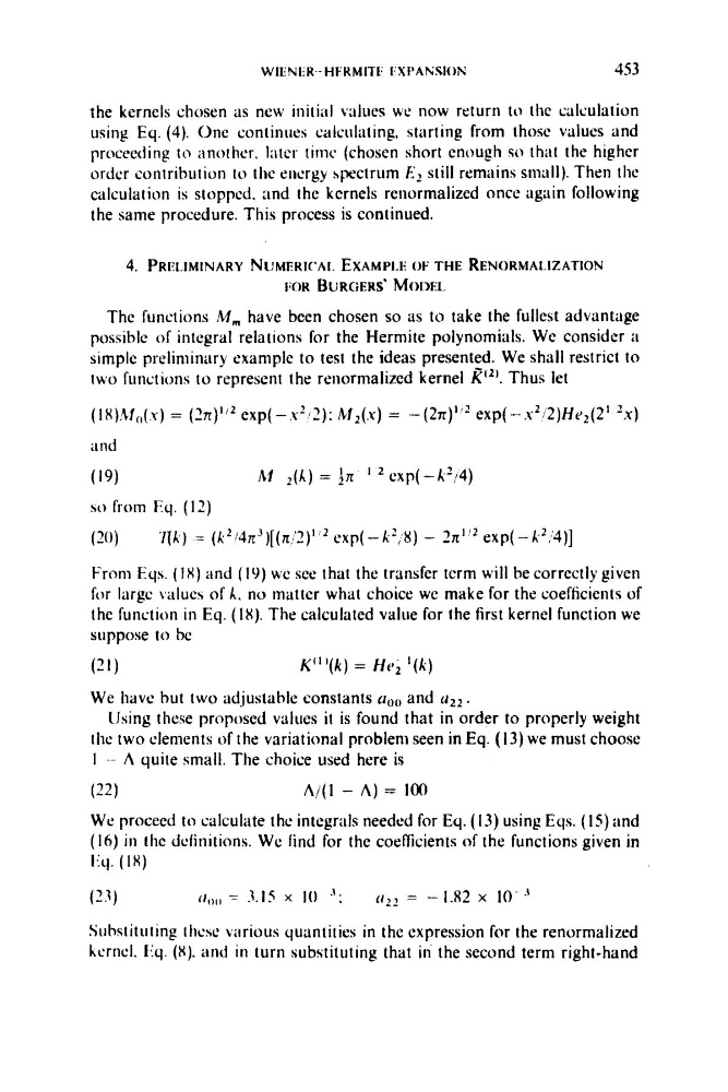
( I R ) , ~ I ( , ( . K ) = (‘n)l’2 exp( - . . Y ’ I ~ ) : M ~ ( . X ) = -(27r)’82 exp( - . ~ ~ : ‘ 2 ) H r , ( 2 ~
‘x)
iind
(19)
hl 2(A) = in ’ CXP( - k ’ j 4 )
so from Eq. (12)
(20)
77kj = (k’/4n”)[(7~i’2)’’~ exp( --A’,,#) - Zn’” exp( -k2;4))1
From Eqs. ( 18) and (19) we see that the transfer term will be correctly given
for large valucs or A, no matter what choice we make for the coefficients of
the function in Eq. (18). The calculated value for the first kernel function we
suppose to be
(21)
K “ ’ ( k ) = He, ‘ ( A )
We have but two adjustable constants uoo and u Z 2 .
llsing these proposed values it is found that in order to properly weight
thc two clements of the variational problem seen in Eq. (13) we must choose
I -- A quite small. The choice used here is
(22)
A / ( l - A ) = 100
We proceed to calculate the integrals needed for Eq. (13) using Eqs. (I5)and
(16) in the dcfinitions. We find for the coefficients o f the functions given in
1,:q. (IR)
(’3)
( I , , , , = 3.15 x I0 ”:
( 1 2 2 = - 1.82 x 10Substituting thcse various quantities in the expression for the renormalized
kernel. I:q. (X). and i n turn substituting that iii the second term right-hand
453
the kernels chosen as new initial v:rlues we now return t o the ciilculation
using Eq. (4). One continues calciilating, starting from those values and
proceeding to another. I;iter timc (chosen short enough s o thilt the higher
order contribution t o tlic energy spectrum E , still remains smt~ll). Then the
calculation is stopped. and the kcrnels renormalized once again following
the same procedure. This process is continued.
4. PRI;:l.IMINARY NUMEKICAI. EXAMPIJ: OF THE RENORMALIZATION
I;OW BURGERS’ MODEL
The functions hl,,, have bcen chosen so as to take the fullest advantage
possible of integral relations for the Hermite polynomials. We consider ;I
simple preliminary example to test the ideas presented. We shall restrict to
two functions to represent the renormalized kernel R”’. Thus let
( I R ) , ~ I ( , ( . K ) = (‘n)l’2 exp( - . . Y ’ I ~ ) : M ~ ( . X ) = -(27r)’82 exp( - . ~ ~ : ‘ 2 ) H r , ( 2 ~
‘x)
iind
(19)
hl 2(A) = in ’ CXP( - k ’ j 4 )
so from Eq. (12)
(20)
77kj = (k’/4n”)[(7~i’2)’’~ exp( --A’,,#) - Zn’” exp( -k2;4))1
From Eqs. ( 18) and (19) we see that the transfer term will be correctly given
for large valucs or A, no matter what choice we make for the coefficients of
the function in Eq. (18). The calculated value for the first kernel function we
suppose to be
(21)
K “ ’ ( k ) = He, ‘ ( A )
We have but two adjustable constants uoo and u Z 2 .
llsing these proposed values it is found that in order to properly weight
thc two clements of the variational problem seen in Eq. (13) we must choose
I -- A quite small. The choice used here is
(22)
A / ( l - A ) = 100
We proceed to calculate the integrals needed for Eq. (13) using Eqs. (I5)and
(16) in the dcfinitions. We find for the coefficients o f the functions given in
1,:q. (IR)
(’3)
( I , , , , = 3.15 x I0 ”:
( 1 2 2 = - 1.82 x 10Substituting thcse various quantities in the expression for the renormalized
kernel. I:q. (X). and i n turn substituting that iii the second term right-hand