

346
GUNNAR KUILENBERG
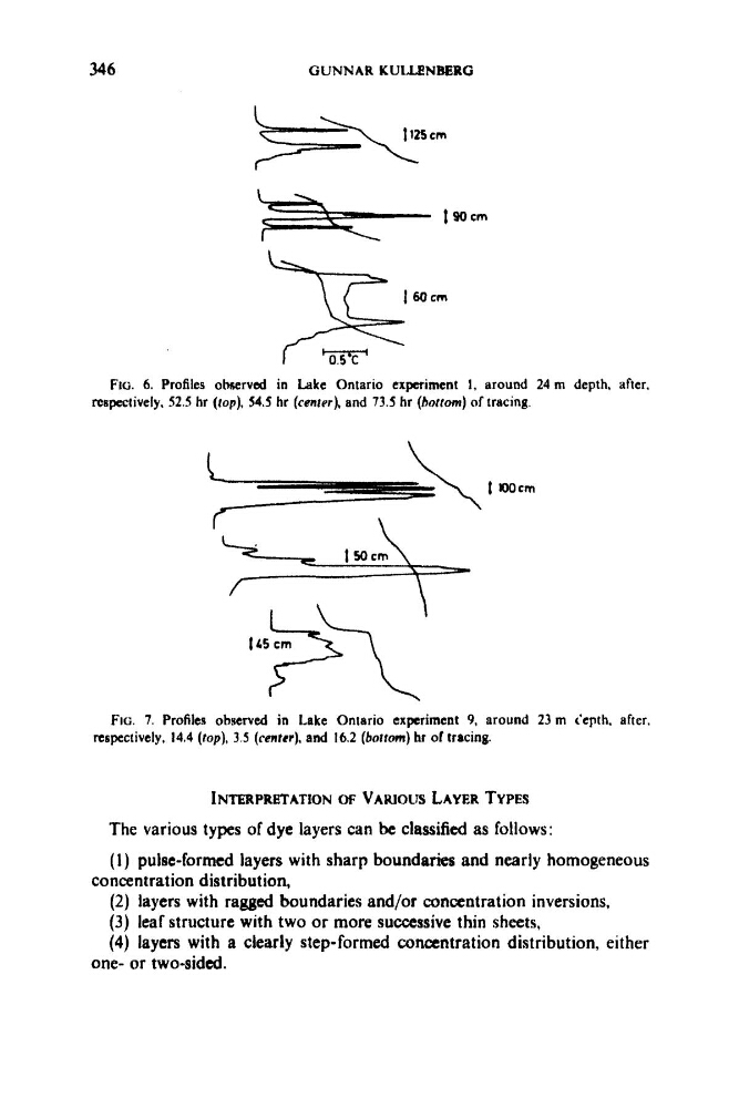
FIG. 6. Profiles observed in Lake Ontario experiment 1, around 24 rn depth, after.
respectively. 52.5 hr (fop), 54.5 hr (cenrur), and 73.5 hr (hotrom) of tracing.
FIG. 7. Profiles observed in Lake Ontario experiment 9, around 23 m depth. after,
respectively, 14.4 (fop), 3.5 (cenrer). and 16.2 (bottom) hr of tracing.
INTERPRETATION w VARJOUS LAYER TYPES
The various types of dye layers can be classified as follows:
( I ) pulse-formed layers with sharp boundaries and nearly homogeneous
(2) layers with ragged boundaries and/or concentration inversions,
(3) leaf structure with two or more successive thin sheets,
(4) layers with a clearly step-formed concentration distribution, either
concentration distribution,
one- or two-sided.
GUNNAR KUILENBERG
FIG. 6. Profiles observed in Lake Ontario experiment 1, around 24 rn depth, after.
respectively. 52.5 hr (fop), 54.5 hr (cenrur), and 73.5 hr (hotrom) of tracing.
FIG. 7. Profiles observed in Lake Ontario experiment 9, around 23 m depth. after,
respectively, 14.4 (fop), 3.5 (cenrer). and 16.2 (bottom) hr of tracing.
INTERPRETATION w VARJOUS LAYER TYPES
The various types of dye layers can be classified as follows:
( I ) pulse-formed layers with sharp boundaries and nearly homogeneous
(2) layers with ragged boundaries and/or concentration inversions,
(3) leaf structure with two or more successive thin sheets,
(4) layers with a clearly step-formed concentration distribution, either
concentration distribution,
one- or two-sided.