

240
A. I IONAHD
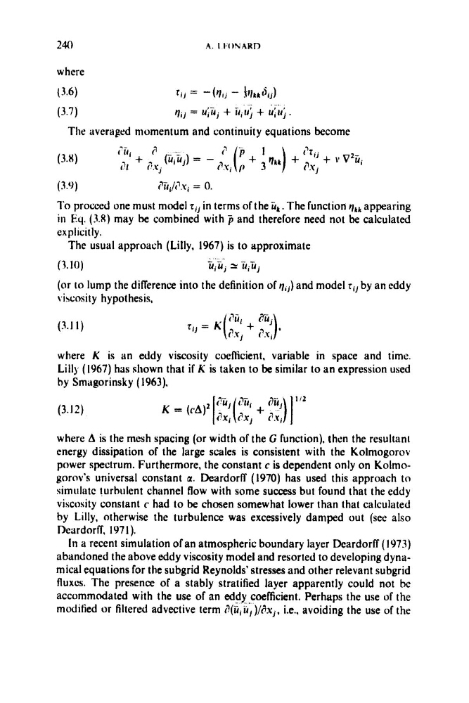
where
(3.6)
r i j = - ( q l j - f r l k k 3 i j )
.
. ~ .
(3.7)
qii = uIUj + idii4j + uluj .
The averaged momentum and continuity equations become
(3.4)
?iii/Cxl = 0.
To proaed one must model ' l i j in terms of the ik. The function q&k appearing
in Eq. (3.8) may be combined with p and therefore need not be calculated
explicitly.
The usual approach (Lilly, 1967) is to approximate
- -
u , u . -v 5.2.
(or to lump the difference into the definition of q,,) and model Ti, by an eddy
viscosity hypothesis,
(3.10)
I J
I J
(3.1 1)
where K is an eddy viscosity coefficient, variable in space and time.
Lilly (1967) has shown that if K is taken to be similar to an expression used
by Smagorinsky (1963).
(3.12)
where A is the mesh spacing (or width of the G function), then the resultant
energy dissipation of the large scales is consistent with the Kolmogorov
power spectrum. Furthermore, the constant c is dependent only on Kolmogorov's universal constant a. Deardorff (1970) has used this approach to
sirniilatc turbulent channel flow with some success but found that the eddy
viscosity constant c had to be chosen somewhat lower than that calculated
by Lilly, otherwise the turbulence was excessively damped out (see also
Deardorff, 197 I ).
In a recent simulation of an atmospheric boundary layer Deardorff (1973)
abandoned the above oddy viscosity model and resorted to developing dynamica1 equations for the subgrid Reynolds' stresses and other relevant subgrid
fluxcs. The presence of a stably stratified layer apparently could not be
accommodated with the use of an eddy coefficient. Perhaps the use of the
moditied or filtered advective term d(iiii)/i?xj, i.e., avoiding the use of the
A. I IONAHD
where
(3.6)
r i j = - ( q l j - f r l k k 3 i j )
.
. ~ .
(3.7)
qii = uIUj + idii4j + uluj .
The averaged momentum and continuity equations become
(3.4)
?iii/Cxl = 0.
To proaed one must model ' l i j in terms of the ik. The function q&k appearing
in Eq. (3.8) may be combined with p and therefore need not be calculated
explicitly.
The usual approach (Lilly, 1967) is to approximate
- -
u , u . -v 5.2.
(or to lump the difference into the definition of q,,) and model Ti, by an eddy
viscosity hypothesis,
(3.10)
I J
I J
(3.1 1)
where K is an eddy viscosity coefficient, variable in space and time.
Lilly (1967) has shown that if K is taken to be similar to an expression used
by Smagorinsky (1963).
(3.12)
where A is the mesh spacing (or width of the G function), then the resultant
energy dissipation of the large scales is consistent with the Kolmogorov
power spectrum. Furthermore, the constant c is dependent only on Kolmogorov's universal constant a. Deardorff (1970) has used this approach to
sirniilatc turbulent channel flow with some success but found that the eddy
viscosity constant c had to be chosen somewhat lower than that calculated
by Lilly, otherwise the turbulence was excessively damped out (see also
Deardorff, 197 I ).
In a recent simulation of an atmospheric boundary layer Deardorff (1973)
abandoned the above oddy viscosity model and resorted to developing dynamica1 equations for the subgrid Reynolds' stresses and other relevant subgrid
fluxcs. The presence of a stably stratified layer apparently could not be
accommodated with the use of an eddy coefficient. Perhaps the use of the
moditied or filtered advective term d(iiii)/i?xj, i.e., avoiding the use of the