

Now. from Eqs. (lo)-( 12), if we knew the distributions of u i u j , Oui and the
value of q/7;, for all time and space, we would know3 Li, and 0 ; having U i
and 0. together with u , u j , urtlg/To, and 8, Eq. (12) would give us the transport terni plus A,, . Thus it must bc possible to write the sum of A,, and the
transport term as a functional of uiuj , Uir; , t;. g;"lb (the latter occurring with
and without &). The trace of the transport term itself may be so written [by
applying the same reasoning to the trace of Eq. (12). since Aii = 01. It is
surely a small step to assume that the tcihole transport term may be so
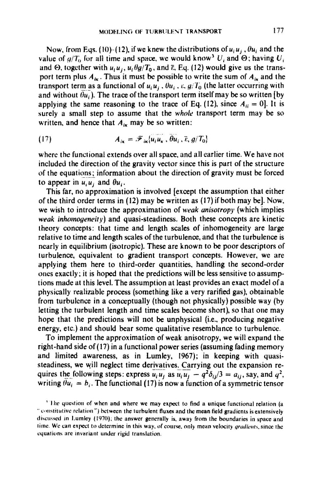
written. and hence that Ai, may be so written:
.
(17)
Ai, = .9i,(uiu, ,014; ,-i, giT,J
where the functional extends over all space, and all earlier time. We have not
included the direction of the gravity vector since this is part of the structure
of the equations; information about the direction of gravity must be forced
to appear in u
:
.
; and hi.
This far, no approximation is involved [except the assumption that either
of the third order terms in (12) may be written as ( I 7) if both may be]. Now,
we wish to introduce the approximation of weak unisorropy (which implies
weak inhornogeneirg) and quasi-steadiness. Both these concepts are kinetic
theory concepts: that time and length scales of inhomogeneity are large
relative to time and length scales of the turbulence, and that the turbulence is
nearly in equilibrium (isotropic). These are known to be poor descriptors of
turbulence, equivalent to gradient transport concepts. However, we are
applying them here to third-order quantities, handling the second-order
ones exactly; it is hoped that the predictions will be less sensitive to assumptions made at this level. The assumption at least provides an exact model of a
physically realizable process (something like a very rarified gas), obtainable
from turbulence in a conceptually (though not physically) possible way (by
letting the turbulent length and time scales become short), so that one may
hope that the predictions will not be unphysical (i.e., producing negative
energy, etc.) and should bear some qualitative resemblance to turbulence.
To implement the approximation of weak anisotropy, we will expand the
right-hand side of (17) in a functional power series (assuming fading memory
and limited awareness, as in Lumley, 1967); in keeping with quasisteadiness, we will neglect time derivatives. .... Carrying -
out the expansion requires the following steps: express uiu, as uiu, - q2Si,/3 = a i j , say, and yz,
writing d i i = h i . The functional (17) is now a function ofa symmetric tensor
' 'I Iir qticstioii of when snd where we may expect to find H unique functional relation (a
.' coiristitiitivc relatirin ") bctween tht turbulent fluxes and the mean tield gradients is extensively
diwusscd in Lumley (IY70); the answer generally is. away from the boundaries in space and
lime. Wc c a l l expcct t o dcterminc in this way. of course. only mean velocity yrcrdicnrs. since the
cquaiions tire invariant under rigid translation.
value of q/7;, for all time and space, we would know3 Li, and 0 ; having U i
and 0. together with u , u j , urtlg/To, and 8, Eq. (12) would give us the transport terni plus A,, . Thus it must bc possible to write the sum of A,, and the
transport term as a functional of uiuj , Uir; , t;. g;"lb (the latter occurring with
and without &). The trace of the transport term itself may be so written [by
applying the same reasoning to the trace of Eq. (12). since Aii = 01. It is
surely a small step to assume that the tcihole transport term may be so
written. and hence that Ai, may be so written:
.
(17)
Ai, = .9i,(uiu, ,014; ,-i, giT,J
where the functional extends over all space, and all earlier time. We have not
included the direction of the gravity vector since this is part of the structure
of the equations; information about the direction of gravity must be forced
to appear in u
:
.
; and hi.
This far, no approximation is involved [except the assumption that either
of the third order terms in (12) may be written as ( I 7) if both may be]. Now,
we wish to introduce the approximation of weak unisorropy (which implies
weak inhornogeneirg) and quasi-steadiness. Both these concepts are kinetic
theory concepts: that time and length scales of inhomogeneity are large
relative to time and length scales of the turbulence, and that the turbulence is
nearly in equilibrium (isotropic). These are known to be poor descriptors of
turbulence, equivalent to gradient transport concepts. However, we are
applying them here to third-order quantities, handling the second-order
ones exactly; it is hoped that the predictions will be less sensitive to assumptions made at this level. The assumption at least provides an exact model of a
physically realizable process (something like a very rarified gas), obtainable
from turbulence in a conceptually (though not physically) possible way (by
letting the turbulent length and time scales become short), so that one may
hope that the predictions will not be unphysical (i.e., producing negative
energy, etc.) and should bear some qualitative resemblance to turbulence.
To implement the approximation of weak anisotropy, we will expand the
right-hand side of (17) in a functional power series (assuming fading memory
and limited awareness, as in Lumley, 1967); in keeping with quasisteadiness, we will neglect time derivatives. .... Carrying -
out the expansion requires the following steps: express uiu, as uiu, - q2Si,/3 = a i j , say, and yz,
writing d i i = h i . The functional (17) is now a function ofa symmetric tensor
' 'I Iir qticstioii of when snd where we may expect to find H unique functional relation (a
.' coiristitiitivc relatirin ") bctween tht turbulent fluxes and the mean tield gradients is extensively
diwusscd in Lumley (IY70); the answer generally is. away from the boundaries in space and
lime. Wc c a l l expcct t o dcterminc in this way. of course. only mean velocity yrcrdicnrs. since the
cquaiions tire invariant under rigid translation.