

I 76
1. L. LCIMLEY A N D R. KHAJEH-NOURI
3. MODELING THE THIRD MOMENTS
If we consistently apply the Reynolds/Peclet number order of magnitude
analysis given here, we obtain thc set of equations given below. [In addition
lo ( I ) and (7). we are considering here only velocity and temperature; the
treatment of a passive contaminant, or of an active contaminant other than
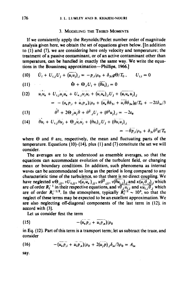
temperature, can be handled in exactly the same way. We write the equations in the Boussinesq approximation-Phillip, 1966.)
(10)
(1 1)
0, + u,,,u, + (UiUi).j = -pJpo + 6,,g@/T, 9 ui.i = 0
6 + O,,ui + (&Ji = 0
-~
= - ( i i p , i + u ~ P , ) / P , + ( U i 8 ~ 3 i
+ U J S ~ , ~ / T O + -2&5iN/3
ii’j + mjujR + iij,ju, + (02u,).,i = -2E,
- .
(13)
(14)
(hi + Ui,,Ou, t O,,iiu, t ( h i ) . j U , + ( O U , U ~ ) . ~
= -Opli/po + S3,Uig/To
where 0 and 8 are, respectively, the mean and fluctuating parts of the
temperature. Equations (lO)-(l4), plus ( I ) and (7) constitute the set we will
consider.
The averages are to be understood as ensemble averages, so that the
equations can accommodate evolution of the turbulent field, or changing
meail or boundary conditions. In addition, such phenomena as internal
waves can be accommodated so long as the period is long compared to any
characteristic time of the turbulence, so that t h e r e n o direct coupling. We
have neglected K @ , ~ , , vUi,j,, v(uiux),,,, K p , l j , ~ ( f k ~ , , ) , ~
and K(i$,,)aj which
are of order R; in their respective equations, and v
6 and K=
which
are of order R;’la. In the atmosphere, typically R:’2 - lo3. so that the
neglect of these terms may be expected to be an excellent approximation. We
are also neglecting offdiagonal components of the last term in (12), in
accord with (3).
Let us consider first the term
-. - -.
I
(15)
- ( U c P , i + uiP.x)/P,
in Eq. (12). Part of this term is a transport term; let us subtract the trace, and
consider
(16)
-(UTi:i 4- Ui&)/po + 2(u,;).,6iK/3po = Ai,
say.
1. L. LCIMLEY A N D R. KHAJEH-NOURI
3. MODELING THE THIRD MOMENTS
If we consistently apply the Reynolds/Peclet number order of magnitude
analysis given here, we obtain thc set of equations given below. [In addition
lo ( I ) and (7). we are considering here only velocity and temperature; the
treatment of a passive contaminant, or of an active contaminant other than
temperature, can be handled in exactly the same way. We write the equations in the Boussinesq approximation-Phillip, 1966.)
(10)
(1 1)
0, + u,,,u, + (UiUi).j = -pJpo + 6,,g@/T, 9 ui.i = 0
6 + O,,ui + (&Ji = 0
-~
= - ( i i p , i + u ~ P , ) / P , + ( U i 8 ~ 3 i
+ U J S ~ , ~ / T O + -2&5iN/3
ii’j + mjujR + iij,ju, + (02u,).,i = -2E,
- .
(13)
(14)
(hi + Ui,,Ou, t O,,iiu, t ( h i ) . j U , + ( O U , U ~ ) . ~
= -Opli/po + S3,Uig/To
where 0 and 8 are, respectively, the mean and fluctuating parts of the
temperature. Equations (lO)-(l4), plus ( I ) and (7) constitute the set we will
consider.
The averages are to be understood as ensemble averages, so that the
equations can accommodate evolution of the turbulent field, or changing
meail or boundary conditions. In addition, such phenomena as internal
waves can be accommodated so long as the period is long compared to any
characteristic time of the turbulence, so that t h e r e n o direct coupling. We
have neglected K @ , ~ , , vUi,j,, v(uiux),,,, K p , l j , ~ ( f k ~ , , ) , ~
and K(i$,,)aj which
are of order R; in their respective equations, and v
6 and K=
which
are of order R;’la. In the atmosphere, typically R:’2 - lo3. so that the
neglect of these terms may be expected to be an excellent approximation. We
are also neglecting offdiagonal components of the last term in (12), in
accord with (3).
Let us consider first the term
-. - -.
I
(15)
- ( U c P , i + uiP.x)/P,
in Eq. (12). Part of this term is a transport term; let us subtract the trace, and
consider
(16)
-(UTi:i 4- Ui&)/po + 2(u,;).,6iK/3po = Ai,
say.