

148
RICHARD L. PESlilN
I I ,
0
2
4
6
8 1 0 I2 14 I6
T I M E
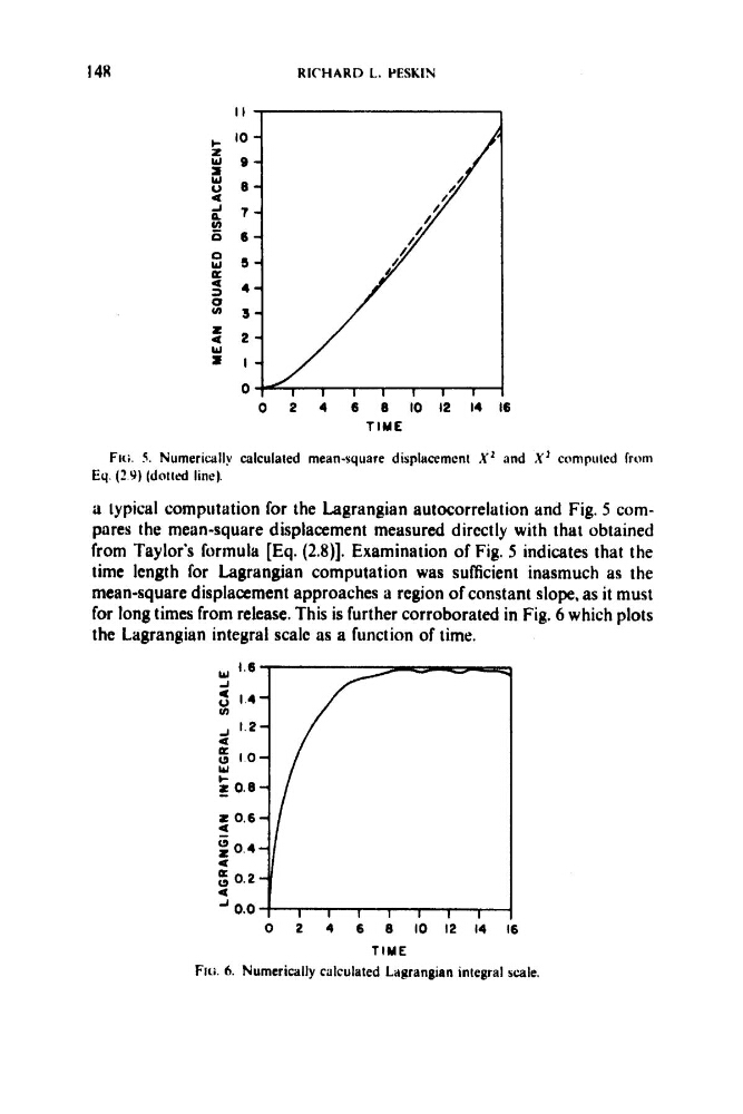
FIG. 5. Numerically calculated mean-square displaccmcnt X’ and X’ computed froin
Eq. (2 9) (dottcd line).
B typical computation for the Lagrangian autocorrelation and Fig. 5 compares the mean-square displacement measured directly with that obtained
from Taylor’s forrnula [Eq. (2.8)]. Examination of Fig. 5 indicates that the
time length for Lagrangian computation was sufficient inasmuch as the
mean-square displacement approaches a region of constant slope, as it must
for long times from release. This is further corroborated in Fig. 6 which plots
the Lagrangian integral scale as a function of time.
1.6 .
; 0.8
2 0.6
$ 0.4
4
4
g
; : y
P 0.2
- 0
.
0
-
0
2
4
6
8
1 O I 2 1 4
T I M E
5
Fici. 6. Numerically calculated Lagrangian integral scale.
RICHARD L. PESlilN
I I ,
0
2
4
6
8 1 0 I2 14 I6
T I M E
FIG. 5. Numerically calculated mean-square displaccmcnt X’ and X’ computed froin
Eq. (2 9) (dottcd line).
B typical computation for the Lagrangian autocorrelation and Fig. 5 compares the mean-square displacement measured directly with that obtained
from Taylor’s forrnula [Eq. (2.8)]. Examination of Fig. 5 indicates that the
time length for Lagrangian computation was sufficient inasmuch as the
mean-square displacement approaches a region of constant slope, as it must
for long times from release. This is further corroborated in Fig. 6 which plots
the Lagrangian integral scale as a function of time.
1.6 .
; 0.8
2 0.6
$ 0.4
4
4
g
; : y
P 0.2
- 0
.
0
-
0
2
4
6
8
1 O I 2 1 4
T I M E
5
Fici. 6. Numerically calculated Lagrangian integral scale.