

Nl.!MERlCAL SIMULATION Of: IAGRAKGIAN QUANTITIES
I47
- 0 . 2 -
- 0 . 4 -
- 0 . 6
9
8
7
6
5
* 4
3
2
I
0
- I
I
I
I
I
1
1
I
~1 I
1
1
1
1
1
1
1
1
1
1
- I
0 I 2 3 4 5 6 7 8 I
X
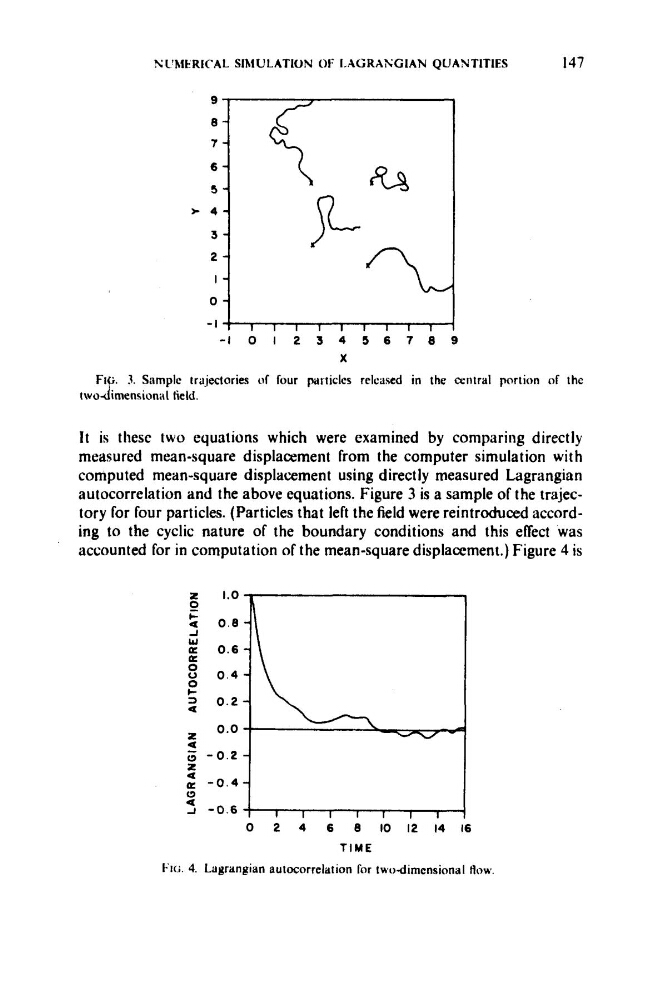
Fip. 3. Simple trajectories of four particles released in the central portion of the
twoJimensionaI field.
It is these two equations which were examined by comparing directly
measured mean-square displacement from the computer simulation with
computed mean-square displacement using directly measured Lagrangian
autocorrelation and the above equations. Figure 3 is a sample of the trajectory for four particles. (Particles that left the field were reintroduced according to the cyclic nature of the boundary conditions and this effect was
accounted for in computation of the mean-square displacement.) Figure 4 is
i
J
c
3
a
z
0
2
4
(3
J
a
-
a
a
Flcj. 4.
I47
- 0 . 2 -
- 0 . 4 -
- 0 . 6
9
8
7
6
5
* 4
3
2
I
0
- I
I
I
I
I
1
1
I
~1 I
1
1
1
1
1
1
1
1
1
1
- I
0 I 2 3 4 5 6 7 8 I
X
Fip. 3. Simple trajectories of four particles released in the central portion of the
twoJimensionaI field.
It is these two equations which were examined by comparing directly
measured mean-square displacement from the computer simulation with
computed mean-square displacement using directly measured Lagrangian
autocorrelation and the above equations. Figure 3 is a sample of the trajectory for four particles. (Particles that left the field were reintroduced according to the cyclic nature of the boundary conditions and this effect was
accounted for in computation of the mean-square displacement.) Figure 4 is
i
J
c
3
a
z
0
2
4
(3
J
a
-
a
a
Flcj. 4.