

383
Testing the Plate Tectonics Model
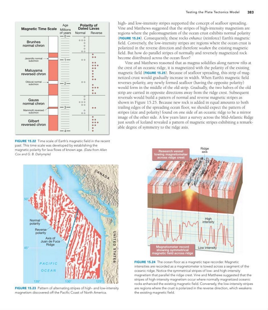
high- and low-intensity stripes supported the concept of seafloor spreading.
Vine and Matthews suggested that the stripes of high-intensity magnetism are
regions where the paleomagnetism of the ocean crust exhibits normal polarity
(FIGURE 15.24). Consequently, these rocks enhance (reinforce) Earth’ s magnetic
field. Conversely, the low-intensity stripes are regions where the ocean crust is
polarized in the reverse direction and therefore weaken the existing magnetic
field. But how do parallel stripes of normally and reversely magnetized rock
become distributed across the ocean floor?
Vine and Matthews reasoned that as magma solidifies along narrow rifts at
the crest of an oceanic ridge, it is magnetized with the polarity of the existing
magnetic field (FIGURE 15.25). Because of seafloor spreading, this strip of magnetized crust would gradually increase in width. When Earth’ s magnetic field
reverses polarity, any newly formed seafloor (having the opposite polarity)
would form in the middle of the old strip. Gradually, the two halves of the old
strip are carried in opposite directions away from the ridge crest. Subsequent
reversals would build a pattern of normal and reverse magnetic stripes as
shown in Figure 15.25. Because new rock is added in equal amounts to both
trailing edges of the spreading ocean floor, we should expect the pattern of
stripes (size and polarity) found on one side of an oceanic ridge to be a mirror
image of the other side. A few years later a survey across the Mid-Atlantic Ridge
just south of Iceland revealed a pattern of magnetic stripes exhibiting a remarkable degree of symmetry to the ridge axis.
Age
Millions
of years Normal
Reverse
1
2
3
4
Brunhes
normal chron
Matuyama
reversed chron
Gauss
normal chron
Gilbert
reversed chron
Jaramillo normal
subchron
Olduvai normal
subchron
Mammoth reversed
subchron
Magnetic Time Scale
Polarity of
Dated Lavas
• •
• • •
• • •
• •
• •
• •
• •
• •
• •
• •
• •
• •
• •
• • •
• • •
• •
• •
• •
• •
• •
• •
• •
• •
• • •
• • •
• •
• •
• •
• •
• •
• •
• •
• •
• •
• • •
• • •
• •
• •
• •
• •
• •
• •
• •
• •
• •
• •
• • •
• • •
• •
• •
• •
• •
0
FIGURE 15.22 Time scale of Earth’s magnetic field in the recent
past. This time scale was developed by establishing the
magnetic polarity for lava flows of known age. (Data from Allen
Cox and G. B. Dalrymple)
C A N A D A
U N I T E D S TAT E S
P A C I F I C
O C E A N
135°
130°
125°
50°
45°
Axis of
Juan de Fuca
Ridge
Normal
polarity
Reverse
polarity
FIGURE 15.23 Pattern of alternating stripes of high- and low-intensity
magnetism discovered off the Pacific Coast of North America.
Magnetometer record
showing symmetrical
magnetic field across ridge
Low intensity
High
intensity
Ridge
axis
Research vessel
towing magnetometer
across ridge crest
FIGURE 15.24 The ocean floor as a magnetic tape recorder. Magnetic
intensities are recorded as a magnetometer is towed across a segment of the
oceanic ridge. Notice the symmetrical stripes of low- and high-intensity
magnetism that parallel the ridge crest. Vine and Matthews suggested that the
stripes of high-intensity magnetism occur where normally magnetized oceanic
rocks enhanced the existing magnetic field. Conversely, the low-intensity stripes
are regions where the crust is polarized in the reverse direction, which weakens
the existing magnetic field.
Testing the Plate Tectonics Model
high- and low-intensity stripes supported the concept of seafloor spreading.
Vine and Matthews suggested that the stripes of high-intensity magnetism are
regions where the paleomagnetism of the ocean crust exhibits normal polarity
(FIGURE 15.24). Consequently, these rocks enhance (reinforce) Earth’ s magnetic
field. Conversely, the low-intensity stripes are regions where the ocean crust is
polarized in the reverse direction and therefore weaken the existing magnetic
field. But how do parallel stripes of normally and reversely magnetized rock
become distributed across the ocean floor?
Vine and Matthews reasoned that as magma solidifies along narrow rifts at
the crest of an oceanic ridge, it is magnetized with the polarity of the existing
magnetic field (FIGURE 15.25). Because of seafloor spreading, this strip of magnetized crust would gradually increase in width. When Earth’ s magnetic field
reverses polarity, any newly formed seafloor (having the opposite polarity)
would form in the middle of the old strip. Gradually, the two halves of the old
strip are carried in opposite directions away from the ridge crest. Subsequent
reversals would build a pattern of normal and reverse magnetic stripes as
shown in Figure 15.25. Because new rock is added in equal amounts to both
trailing edges of the spreading ocean floor, we should expect the pattern of
stripes (size and polarity) found on one side of an oceanic ridge to be a mirror
image of the other side. A few years later a survey across the Mid-Atlantic Ridge
just south of Iceland revealed a pattern of magnetic stripes exhibiting a remarkable degree of symmetry to the ridge axis.
Age
Millions
of years Normal
Reverse
1
2
3
4
Brunhes
normal chron
Matuyama
reversed chron
Gauss
normal chron
Gilbert
reversed chron
Jaramillo normal
subchron
Olduvai normal
subchron
Mammoth reversed
subchron
Magnetic Time Scale
Polarity of
Dated Lavas
• •
• • •
• • •
• •
• •
• •
• •
• •
• •
• •
• •
• •
• •
• • •
• • •
• •
• •
• •
• •
• •
• •
• •
• •
• • •
• • •
• •
• •
• •
• •
• •
• •
• •
• •
• •
• • •
• • •
• •
• •
• •
• •
• •
• •
• •
• •
• •
• •
• • •
• • •
• •
• •
• •
• •
0
FIGURE 15.22 Time scale of Earth’s magnetic field in the recent
past. This time scale was developed by establishing the
magnetic polarity for lava flows of known age. (Data from Allen
Cox and G. B. Dalrymple)
C A N A D A
U N I T E D S TAT E S
P A C I F I C
O C E A N
135°
130°
125°
50°
45°
Axis of
Juan de Fuca
Ridge
Normal
polarity
Reverse
polarity
FIGURE 15.23 Pattern of alternating stripes of high- and low-intensity
magnetism discovered off the Pacific Coast of North America.
Magnetometer record
showing symmetrical
magnetic field across ridge
Low intensity
High
intensity
Ridge
axis
Research vessel
towing magnetometer
across ridge crest
FIGURE 15.24 The ocean floor as a magnetic tape recorder. Magnetic
intensities are recorded as a magnetometer is towed across a segment of the
oceanic ridge. Notice the symmetrical stripes of low- and high-intensity
magnetism that parallel the ridge crest. Vine and Matthews suggested that the
stripes of high-intensity magnetism occur where normally magnetized oceanic
rocks enhanced the existing magnetic field. Conversely, the low-intensity stripes
are regions where the crust is polarized in the reverse direction, which weakens
the existing magnetic field.