

speleothem
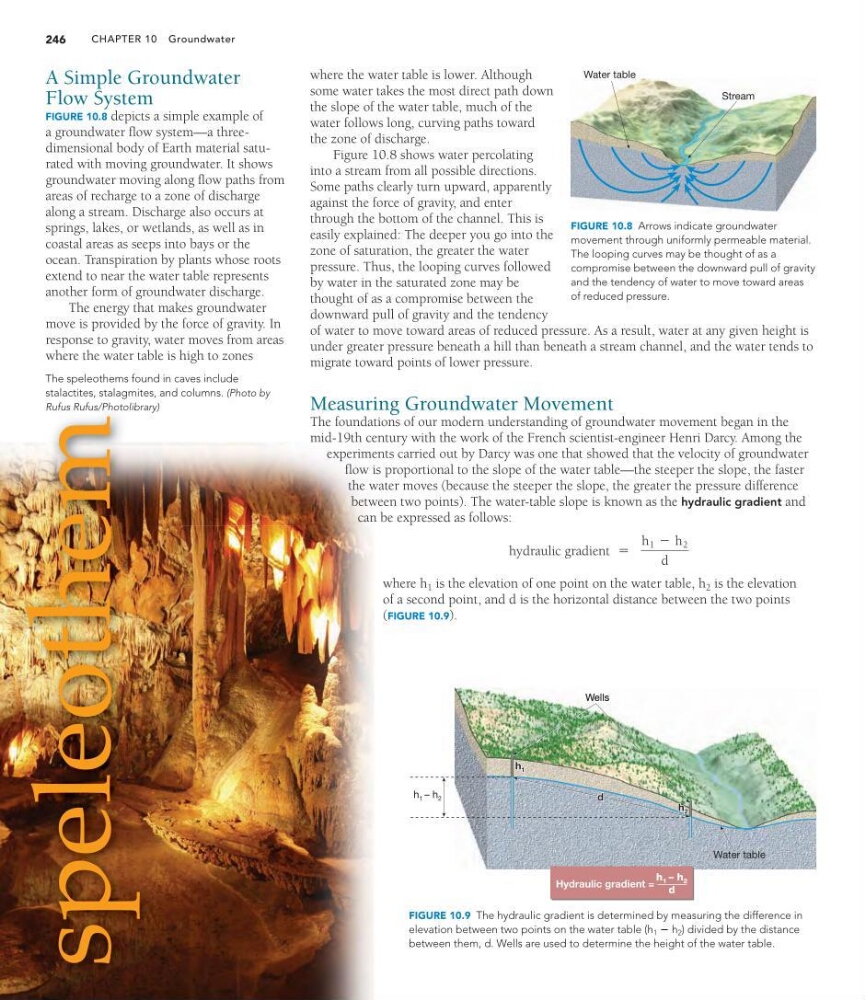
The speleothems found in caves include
stalactites, stalagmites, and columns. (Photo by
Rufus Rufus/Photolibrary)
where the water table is lower. Although
some water takes the most direct path down
the slope of the water table, much of the
water follows long, curving paths toward
the zone of discharge.
Figure 10.8 shows water percolating
into a stream from all possible directions.
Some paths clearly turn upward, apparently
against the force of gravity, and enter
through the bottom of the channel. This is
easily explained: The deeper you go into the
zone of saturation, the greater the water
pressure. Thus, the looping curves followed
by water in the saturated zone may be
thought of as a compromise between the
downward pull of gravity and the tendency
of water to move toward areas of reduced pressure. As a result, water at any given height is
under greater pressure beneath a hill than beneath a stream channel, and the water tends to
migrate toward points of lower pressure.
Measuring Groundwater Movement
The foundations of our modern understanding of groundwater movement began in the
mid-19th century with the work of the French scientist-engineer Henri Darcy. Among the
experiments carried out by Darcy was one that showed that the velocity of groundwater
flow is proportional to the slope of the water table—the steeper the slope, the faster
the water moves (because the steeper the slope, the greater the pressure difference
between two points). The water-table slope is known as the hydraulic gradient and
can be expressed as follows:
where h 1 is the elevation of one point on the water table, h 2 is the elevation
of a second point, and d is the horizontal distance between the two points
(FIGURE 10.9).
hydraulic gradient =
h 1 - h 2
d
CHAPTER 10 Groundwater
246
Stream
Water table
FIGURE 10.8 Arrows indicate groundwater
movement through uniformly permeable material.
The looping curves may be thought of as a
compromise between the downward pull of gravity
and the tendency of water to move toward areas
of reduced pressure.
A Simple Groundwater
Flow System
FIGURE 10.8 depicts a simple example of
a groundwater flow system—a threedimensional body of Earth material saturated with moving groundwater. It shows
groundwater moving along flow paths from
areas of recharge to a zone of discharge
along a stream. Discharge also occurs at
springs, lakes, or wetlands, as well as in
coastal areas as seeps into bays or the
ocean. Transpiration by plants whose roots
extend to near the water table represents
another form of groundwater discharge.
The energy that makes groundwater
move is provided by the force of gravity. In
response to gravity, water moves from areas
where the water table is high to zones
h 1 – h 2
d
h 1 – h 2
h 2
h 1
d
h 2
h 1
d
Wells
Water table
Wells
Hydraulic gradient =
FIGURE 10.9 The hydraulic gradient is determined by measuring the difference in
elevation between two points on the water table (h 1 2 h 2 ) divided by the distance
between them, d. Wells are used to determine the height of the water table.
The speleothems found in caves include
stalactites, stalagmites, and columns. (Photo by
Rufus Rufus/Photolibrary)
where the water table is lower. Although
some water takes the most direct path down
the slope of the water table, much of the
water follows long, curving paths toward
the zone of discharge.
Figure 10.8 shows water percolating
into a stream from all possible directions.
Some paths clearly turn upward, apparently
against the force of gravity, and enter
through the bottom of the channel. This is
easily explained: The deeper you go into the
zone of saturation, the greater the water
pressure. Thus, the looping curves followed
by water in the saturated zone may be
thought of as a compromise between the
downward pull of gravity and the tendency
of water to move toward areas of reduced pressure. As a result, water at any given height is
under greater pressure beneath a hill than beneath a stream channel, and the water tends to
migrate toward points of lower pressure.
Measuring Groundwater Movement
The foundations of our modern understanding of groundwater movement began in the
mid-19th century with the work of the French scientist-engineer Henri Darcy. Among the
experiments carried out by Darcy was one that showed that the velocity of groundwater
flow is proportional to the slope of the water table—the steeper the slope, the faster
the water moves (because the steeper the slope, the greater the pressure difference
between two points). The water-table slope is known as the hydraulic gradient and
can be expressed as follows:
where h 1 is the elevation of one point on the water table, h 2 is the elevation
of a second point, and d is the horizontal distance between the two points
(FIGURE 10.9).
hydraulic gradient =
h 1 - h 2
d
CHAPTER 10 Groundwater
246
Stream
Water table
FIGURE 10.8 Arrows indicate groundwater
movement through uniformly permeable material.
The looping curves may be thought of as a
compromise between the downward pull of gravity
and the tendency of water to move toward areas
of reduced pressure.
A Simple Groundwater
Flow System
FIGURE 10.8 depicts a simple example of
a groundwater flow system—a threedimensional body of Earth material saturated with moving groundwater. It shows
groundwater moving along flow paths from
areas of recharge to a zone of discharge
along a stream. Discharge also occurs at
springs, lakes, or wetlands, as well as in
coastal areas as seeps into bays or the
ocean. Transpiration by plants whose roots
extend to near the water table represents
another form of groundwater discharge.
The energy that makes groundwater
move is provided by the force of gravity. In
response to gravity, water moves from areas
where the water table is high to zones
h 1 – h 2
d
h 1 – h 2
h 2
h 1
d
h 2
h 1
d
Wells
Water table
Wells
Hydraulic gradient =
FIGURE 10.9 The hydraulic gradient is determined by measuring the difference in
elevation between two points on the water table (h 1 2 h 2 ) divided by the distance
between them, d. Wells are used to determine the height of the water table.