

5.4 PALEOCURRENT ANALYSIS
171
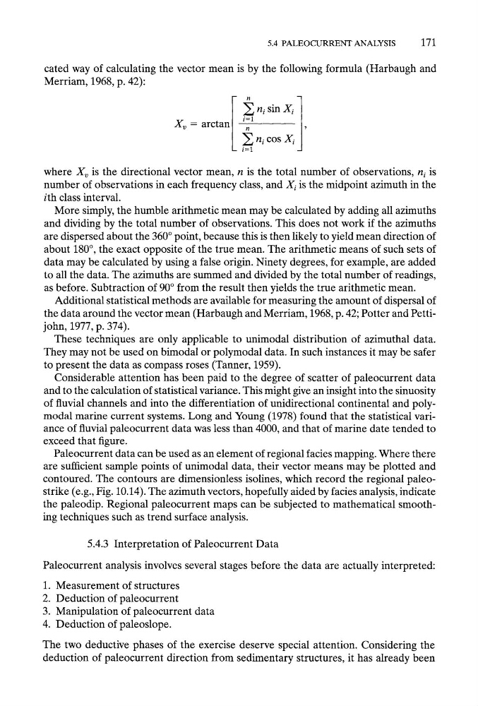
cated way of calculating the vector mean is by the following formula (Harbaugh and
Merriam, 1968, p. 42):
• n i sin Xi
i=1
X~ = arctan
'
H i COS X i
i=1
where X~ is the directional vector mean, n is the total number of observations, ni is
number of observations in each frequency class, and Xg is the midpoint azimuth in the
ith class interval.
More simply, the humble arithmetic mean may be calculated by adding all azimuths
and dividing by the total number of observations. This does not work if the azimuths
are dispersed about the 360 ~ point, because this is then likely to yield mean direction of
about 180 ~ , the exact opposite of the true mean. The arithmetic means of such sets of
data may be calculated by using a false origin. Ninety degrees, for example, are added
to all the data. The azimuths are summed and divided by the total number of readings,
as before. Subtraction of 90 ~ from the result then yields the true arithmetic mean.
Additional statistical methods are available for measuring the amount of dispersal of
the data around the vector mean (Harbaugh and Merriam, 1968, p. 42; Potter and Pettijohn, 1977, p. 374).
These techniques are only applicable to unimodal distribution of azimuthal data.
They may not be used on bimodal or polymodal data. In such instances it may be safer
to present the data as compass roses (Tanner, 1959).
Considerable attention has been paid to the degree of scatter of paleocurrent data
and to the calculation of statistical variance. This might give an insight into the sinuosity
of fluvial channels and into the differentiation of unidirectional continental and polymodal marine current systems. Long and Young (1978) found that the statistical variance of fluvial paleocurrent data was less than 4000, and that of marine date tended to
exceed that figure.
Paleocurrent data can be used as an element of regional facies mapping. Where there
are sufficient sample points of unimodal data, their vector means may be plotted and
contoured. The contours are dimensionless isolines, which record the regional paleostrike (e.g., Fig. 10.14). The azimuth vectors, hopefully aided by facies analysis, indicate
the paleodip. Regional paleocurrent maps can be subjected to mathematical smoothing techniques such as trend surface analysis.
5.4.3 Interpretation of Paleocurrent Data
Paleocurrent analysis involves several stages before the data are actually interpreted:
1. Measurement of structures
2. Deduction of paleocurrent
3. Manipulation of paleocurrent data
4. Deduction of paleoslope.
The two deductive phases of the exercise deserve special attention. Considering the
deduction of paleocurrent direction from sedimentary structures, it has already been
171
cated way of calculating the vector mean is by the following formula (Harbaugh and
Merriam, 1968, p. 42):
• n i sin Xi
i=1
X~ = arctan
'
H i COS X i
i=1
where X~ is the directional vector mean, n is the total number of observations, ni is
number of observations in each frequency class, and Xg is the midpoint azimuth in the
ith class interval.
More simply, the humble arithmetic mean may be calculated by adding all azimuths
and dividing by the total number of observations. This does not work if the azimuths
are dispersed about the 360 ~ point, because this is then likely to yield mean direction of
about 180 ~ , the exact opposite of the true mean. The arithmetic means of such sets of
data may be calculated by using a false origin. Ninety degrees, for example, are added
to all the data. The azimuths are summed and divided by the total number of readings,
as before. Subtraction of 90 ~ from the result then yields the true arithmetic mean.
Additional statistical methods are available for measuring the amount of dispersal of
the data around the vector mean (Harbaugh and Merriam, 1968, p. 42; Potter and Pettijohn, 1977, p. 374).
These techniques are only applicable to unimodal distribution of azimuthal data.
They may not be used on bimodal or polymodal data. In such instances it may be safer
to present the data as compass roses (Tanner, 1959).
Considerable attention has been paid to the degree of scatter of paleocurrent data
and to the calculation of statistical variance. This might give an insight into the sinuosity
of fluvial channels and into the differentiation of unidirectional continental and polymodal marine current systems. Long and Young (1978) found that the statistical variance of fluvial paleocurrent data was less than 4000, and that of marine date tended to
exceed that figure.
Paleocurrent data can be used as an element of regional facies mapping. Where there
are sufficient sample points of unimodal data, their vector means may be plotted and
contoured. The contours are dimensionless isolines, which record the regional paleostrike (e.g., Fig. 10.14). The azimuth vectors, hopefully aided by facies analysis, indicate
the paleodip. Regional paleocurrent maps can be subjected to mathematical smoothing techniques such as trend surface analysis.
5.4.3 Interpretation of Paleocurrent Data
Paleocurrent analysis involves several stages before the data are actually interpreted:
1. Measurement of structures
2. Deduction of paleocurrent
3. Manipulation of paleocurrent data
4. Deduction of paleoslope.
The two deductive phases of the exercise deserve special attention. Considering the
deduction of paleocurrent direction from sedimentary structures, it has already been